

Algorithms and data structures
.pdf7.2 (a, b)-Trees and Red–Black Trees |
153 |
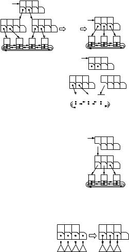
The “leftover” middle key k = s [b + 1 −d] is an upper bound for the keys reachable from t. It and the pointer to t are needed in the predecessor u of v. The situation for u is analogous to the situation for v before the insertion: if v was the i-th child of u, t displaces it to the right. Now t becomes the i-th child, and k is inserted as the i-th splitter. The addition of t as an additional child of u increases the degree of u. If the degree of u becomes b + 1, we split u. The process continues until either some ancestor of v has room to accommodate the new child or the root is split.
In the latter case, we allocate a new root node pointing to the two fragments of the old root. This is the only situation where the height of the tree can increase. In this case, the depth of all leaves increases by one, i.e., we maintain the invariant that all leaves have the same depth. Since the height of the tree is O(log n) (see Lemma 7.1), we obtain a worst-case execution time of O(log n) for insert. Pseudocode is shown in Fig. 7.8.4
We still need to argue that insert leaves us with a correct (a, b)-tree. When we split a node of degree b + 1, we create nodes of degree d = (b + 1)/2 and b + 1 −d. Both degrees are clearly at most b. Also, b + 1 − (b + 1)/2 ≥ a if b ≥ 2a − 1. Convince yourself that b = 2a − 2 will not work.
Exercise 7.6. It is tempting to streamline insert by calling locate to replace the initial descent of the tree. Why does this not work? Would it work if every node had a pointer to its parent?
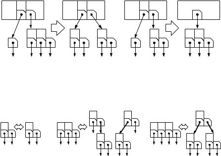
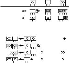
We now turn to the operation remove. The approach is similar to what we already know from our study of insert. We locate the element to be removed, remove it from the sorted list, and repair possible violations of invariants on the way back up. Figure 7.9 shows pseudocode. When a parent u notices that the degree of its child c[i] has dropped to a − 1, it combines this child with one of its neighbors c[i − 1] or c[i + 1] to repair the invariant. There are two cases illustrated in Fig. 7.10. If the neighbor has degree larger than a, we can balance the degrees by transferring some nodes from the neighbor. If the neighbor has degree a, balancing cannot help since both nodes together have only 2a − 1 children, so that we cannot give a children to both of them. However, in this case we can fuse them into a single node, since the requirement b ≥ 2a − 1 ensures that the fused node has degree b at most.
To fuse a node c[i] with its right neighbor c[i + 1], we concatenate their child arrays. To obtain the corresponding splitters, we need to place the splitter s[i] of the parent between the splitter arrays. The fused node replaces c[i+ 1], c[i] is deallocated, and c[i], together with the splitter s[i], is removed from the parent node.
Exercise 7.7. Suppose a node v has been produced by fusing two nodes as described above. Prove that the ordering invariant is maintained: an element e reachable through child v.c[i] has key v.s[i − 1] < key(e) ≤ v.s[i] for 1 ≤ i ≤ v.d.
Balancing two neighbors is equivalent to first fusing them and then splitting the result, as in the operation insert. Since fusing two nodes decreases the degree of their
4 We borrow the notation C :: m from C++ to define a method m for class C.
154 |
7 |
Sorted Sequences |
|
|
|
|
|
|
|
r |
|
3 |
|
// Example: |
2, 3, 5 .remove(5) |
|
|
|
|
|
Procedure ABTree::remove(k : Key) // |
2 |
|
|
5 |
||
|
r.removeRec(k, height, ) |
|
|
k |
|
|
|
if r.d = 1 height > 1 then |
|
|
∞ |
||
|
2 |
3 |
5 |
|||
|
r := r; r := r .c[1]; dispose r |
|
|
|
|
|
Procedure ABItem::removeRec(k : Key, h : N, : List of Element) |
||||||
|
i := locateLocally(k) |
|
|
|
|
|
|
if h = 1 then // base case |
|
|
|
|
|
|
if key(c[i] → e) = k then // there is sth to remove |
|||||
.remove(c[i])
r |
2 3 |
... |
|
2 |
3 ∞ |
//
r
3

 i 2 s
i 2 s
c 
removeLocally(i) |
// |
|
|
|
|
|
|
|
|
|
|
∞ |
|
|
||||||
2 |
|
3 |
|
|
||||||||||||||||
else |
|
|
|
|
|
|
|
|
|
|
|
|
|
|
|
|
|
|
|
|
|
|
|
|
|
|
|
|
|
|
|
|
|
|
|
|
|
|
|
|
|
|
|
|
|
|
|
|
|
|
|
|
|
|
|
|
|
|
|
|
|
|
|
|
|
|
|
|
|
|
|
|
|
|
|
|
|
|
|
|
|
|
|
|
|
|
|
|
|
|
|
|
|
|
|
|
|
|
|
|
|
|
|
|
c[i] → removeRec(e, h − 1, ) |
|
|
|
|
|
|
|
|
|
|
|
|
|
|
|
|
|
|
|
|
|
|
|
|
|
|
|
|
|
|
|
|
|
|
|
|
|
|
|
|
|
if c[i] → d < a then |
// invariant needs repair |
|||||||||||||||||||
if i = d then i-- |
// make sure i and i + 1 are valid neighbors |
|||||||||||||||||||
s := concatenate(c[i] |
→ |
s, s[i] , c[i + 1] |
→ |
s)) |
|
|
|
|
|
|
|
r |
||
|
|
|
|
|
|
|
|
|
|
|
|
|||
c := concatenate(c[i] → c, c[i + 1] → c) |
|
|
|
|
|
|
|
|
|
|
||||
d := |c | |
|
|
|
|
|
|
|
|
|
|
|
|
|
|
if d ≤ b then |
// fuse |
|
|
|
|
|
|
|
|
|
|
|
|
|
(c[i + 1] → s, c[i + 1] → c, c[i + 1] → d) := (s , c , d ) |
|
|
|
|
|
|||||||||
dispose c[i]; removeLocally(i) |
|
|
|
|
|
|
|
// |
|
|||||
else |
// balance |
|
|
|
|
|
|
|
|
|
|
|
|
|
m := d /2 |
|
|
|
|
|
|
|
|
|
|
|
|
|
|
(c[i] → s, c[i] → c, c[i] → d) := (s [1..m − 1], c [1..m], m) |
|
|
|
|||||||||||
(c[i + 1] → s, |
|
|
c[i + 1] → c, |
c[i + 1] → d) := |
||||||||||
(s [m + 1..d − 1], |
c [m + 1..d ], |
d − m) |
|
|
|
|
|
|||||||
s[i] := s [m] |
|
|
|
|
|
|
|
|
|
i |
|
|
|
|
// Remove the i-th child from an ABItem |
|
|
|
|
|
|
|
|
|
|||||
|
|
|
s x |
y |
z |
|||||||||
Procedure ABItem::removeLocally(i : N) |
|
|
c |
|
|
|
|
|
|
|
||||
|
|
|
|
|
|
|
|
|||||||
c[i..d − 1] := c[i + 1..d] |
|
|
|
|
|
|
|
|
|
|
|
|
|
|
|
|
|
|
|
a |
b |
c d |
|||||||
s[i..d − 2] := s[i + 1..d − 1] |
|
|
|
|
// |
|||||||||
|
|
|
|
|
|
|
|
|
|
|
|
|||
d--
 i
i
s
c 
s 2 3 c 

2 3 ∞
i x z
a c d
Fig. 7.9. Removal from an (a, b)-tree
parent, the need to fuse or balance might propagate up the tree. If the degree of the root drops to one, we do one of two things. If the tree has height one and hence contains only a single element, there is nothing to do and we are finished. Otherwise, we deallocate the root and replace it by its sole child. The height of the tree decreases by one.
The execution time of remove is also proportional to the height of the tree and hence logarithmic in the size of the sorted sequence. We summarize the performance of (a, b)-trees in the following theorem.
|
|
|
|
7.2 |
(a, b)-Trees and Red–Black Trees |
155 |
||
|
k1 |
|
k2 |
|
|
k |
|
|
|
k2 |
|
k1 |
|
|
|
k |
|
v |
|
|
v |
|
v |
|
|
|
|
|
|
|
|
|
|
||
c1 |
c2 |
c3 c4 |
c1 c2 |
c3 c4 |
c1 |
c2 c3 |
c1 c2 c3 |
|
Fig. 7.10. Node balancing and fusing in (2,4)-trees: node v has degree a − 1 (here 1). In the situation on the left, it has a sibling of degree a + 1 or more (here 3), and we balance the degrees. In the situation on the right, the sibling has degree a and we fuse v and its sibling. Observe how keys are moved. When two nodes are fused, the degree of the parent decreases
or
Fig. 7.11. The correspondence between (2,4)-trees and red–black trees. Nodes of degree 2, 3, and 4 as shown on the left correspond to the configurations on the right. Red edges are shown in bold
Theorem 7.2. For any integers a and b with a ≥ 2 and b ≥ 2a − 1, (a, b)-trees support the operations insert, remove, and locate on sorted sequences of size n in time
O(log n).
Exercise 7.8. Give a more detailed implementation of locateLocally based on binary search that needs at most log b comparisons. Your code should avoid both explicit use of infinite key values and special case treatments for extreme cases.
Exercise 7.9. Suppose a = 2k and b = 2a. Show that (1 + 1k ) log n + 1 element comparisons suffice to execute a locate operation in an (a, b)-tree. Hint: it is not quite sufficient to combine Exercise 7.4 with Exercise 7.8 since this would give you an additional term +k.
Exercise 7.10. Extend (a, b)-trees so that they can handle multiple occurrences of the same key. Elements with identical keys should be treated last-in first-out, i.e., remove(k) should remove the least recently inserted element with key k.
*Exercise 7.11 (red–black trees). A red–black tree is a binary search tree where the edges are colored either red or black. The black depth of a node v is the number of black edges on the path from the root to v. The following invariants have to hold:

1567 Sorted Sequences
(a)All leaves have the same black depth.
(b)Edges into leaves are black.
(c)No path from the root to a leaf contains two consecutive red edges.
Show that red–black trees and (2, 4)-trees are isomorphic in the following sense: (2, 4)-trees can be mapped to red–black trees by replacing nodes of degree three or four by two or three nodes, respectively, connected by red edges as shown in Fig. 7.11. Red–black trees can be mapped to (2, 4)-trees using the inverse transformation, i.e., components induced by red edges are replaced by a single node. Now explain how to implement (2, 4)-trees using a representation as a red–black tree.5 Explain how the operations of expanding, shrinking, splitting, merging, and balancing nodes of the (2, 4)-tree can be translated into recoloring and rotation operations in the red–black tree. Colors are stored at the target nodes of the corresponding edges.
7.3 More Operations
Search trees support many operations in addition to insert, remove, and locate. We shall study them in two batches. In this section, we shall discuss operations directly supported by (a, b)-trees, and in Sect. 7.5 we shall discuss operations that require augmentation of the data structure.
•min/max. The constant-time operations first and last on a sorted list give us the smallest and the largest element in the sequence in constant time. In particular, search trees implement double-ended priority queues, i.e., sets that allow locating and removing both the smallest and the largest element in logarithmic time. For example, in Fig. 7.5, the dummy element of list gives us access to the smallest element, 2, and to the largest element, 19, via its next and prev pointers, respectively.
•Range queries. To retrieve all elements with keys in the range [x, y], we first locate x and then traverse the sorted list until we see an element with a key larger than y. This takes time O(log n + output size). For example, the range query [4, 14] applied to the search tree in Fig. 7.5 will find the 5, it subsequently outputs 7, 11, 13, and it stops when it sees the 17.
•Build/rebuild. Exercise 7.12 asks you to give an algorithm that converts a sorted list or array into an (a, b)-tree in linear time. Even if we first have to sort the elements, this operation is much faster than inserting the elements one by one. We also obtain a more compact data structure this way.
Exercise 7.12. Explain how to construct an (a, b)-tree from a sorted list in linear time. Which (2, 4)-tree does your routine construct for the sequence 1..17 ? Next, remove the elements 4, 9, and 16.
5 This may be more space-efficient than a direct representation, if the keys are large.
7.3 More Operations |
157 |
7.3.1 *Concatenation
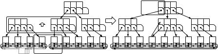
Two sorted sequences can be concatenated if the largest element of the first sequence is smaller than the smallest element of the second sequence. If sequences are represented as (a, b)-trees, two sequences q1 and q2 can be concatenated in time O(log max(|q1|, |q2|)). First, we remove the dummy item from q1 and concatenate the underlying lists. Next, we fuse the root of one tree with an appropriate node of the other tree in such a way that the resulting tree remains sorted and balanced. More precisely, if q1.height ≥ q2.height, we descend q1.height − q2.height levels from the root of q1 by following pointers to the rightmost children. The node v, that we reach is then fused with the root of q2. The new splitter key required is the largest key in q1. If the degree of v now exceeds b, v is split. From that point, the concatenation proceeds like an insert operation, propagating splits up the tree until the invariant is fulfilled or a new root node is created. The case q1.height < q2.height is a mirror image. We descend q2.height − q1.height levels from the root of q2 by following pointers to the leftmost children, and fuse . . . . If we explicitly store the heights of the trees, the operation runs in time O(1 + |q1.height − q2.height|) = O(log(|q1| + |q2|)). Figure 7.12 gives an example.
q1 |
q2 |
17 |
5:insert |
5 |
17 |
|
|
|
|
|
|
|
|
2 3 5 |
4:split 11 13 |
19 |
2 3 |
7 |
11 13 |
19 |
|
3:fuse |
|
|
|
|
|
2 |
3 |
5 |
7 |
11 |
13 |
17 |
19 |
∞ |
2 |
3 |
5 |
7 |
11 |
13 |
17 |
19 |
∞ |
1:delete ∞ |
|
2:concatenate |
|
|
|
|
|
|
|
|
|
|
|
|
|
||
Fig. 7.12. Concatenating (2, 4)-trees for 2, 3, 5, 7 and 11, 13, 17, 19
7.3.2 *Splitting
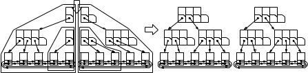
We now show how to split a sorted sequence at a given element in logarithmic time. Consider a sequence q = w, . . . , x, y, . . . , z . Splitting q at y results in the sequences q1 = w, . . . , x and q2 = y, . . . , z . We implement splitting as follows. Consider the path from the root to leaf y. We split each node v on this path into two nodes, v and vr. Node v gets the children of v that are to the left of the path and vr gets the children, that are to the right of the path. Some of these nodes may get no children. Each of the nodes with children can be viewed as the root of an (a, b)-tree. Concatenating the left trees and a new dummy sequence element yields the elements up to x. Concatenating y and the right trees produces the sequence of elements starting from y. We can do these O(log n) concatenations in total time O(log n) by exploiting the fact that the left trees have a strictly decreasing height and the right trees have a strictly increasing height. Let us look at the trees on the left in more detail. Let
158 7 Sorted Sequences
r1, r2 to rk be the roots of the trees on the left and let h1, h2 to hh be their heights. Then h1 ≥ h2 ≥ . . . ≥ hk. We first concatenate rk−1 and rk in time O(1 + hk−1 − hk), then concatenate rk−2 with the result in time O(1 + hk−2 − hk−1), then concatenate rk−3 with the result in time O(1 + hk−2 − hk−1), and so on. The total time needed for all concatenations is O ∑1≤i<k(1 + hi − hi+1) = O(k + h1 − hk) = O(log n). Figure 7.13 gives an example.
Exercise 7.13. We glossed over one issue in the argument above. What is the height of the tree resulting from concatenating the trees with roots rk to ri? Show that the height is hi + O(1).
Exercise 7.14. Explain how to remove a subsequence e q : α ≤ e ≤ β from an (a, b)-tree q in time O(log n).
split < 2, 3, 5, 7, 11, 13, 17, 19 > at 11
2 |
3 |
13 |
19 |
2 3 |
|
5 7 ∞ 11 |
13 17 19 ∞ |
|
|
3 |
|
|
|
13 |
|
|
|
2 |
|
5 |
7 |
|
11 |
17 19 |
|
2 |
3 |
5 |
|
7 |
∞ |
11 13 |
17 19 |
∞ |
Fig. 7.13. Splitting the (2, 4)-tree for 2, 3, 5, 7, 11, 13, 17, 19 shown in Fig. 7.5 produces the subtrees shown on the left. Subsequently concatenating the trees surrounded by the dashed lines leads to the (2, 4)-trees shown on the right
7.4 Amortized Analysis of Update Operations
The best-case time for an insertion or removal is considerably smaller than the worstcase time. In the best case, we basically pay for locating the affected element, for updating the sequence, and for updating the bottommost internal node. The worst case is much slower. Split or fuse operations may propagate all the way up the tree.
Exercise 7.15. Give a sequence of n operations on (2, 3)-trees that requires Ω(n log n) split and fuse operations.
We now show that the amortized complexity is essentially equal to that of the best case if b is not at its minimum possible value but is at least 2a. In Sect. 7.5.1, we shall see variants of insert and remove that turn out to have constant amortized complexity in the light of the analysis below.
Theorem 7.3. Consider an (a, b)-tree with b ≥ 2a that is initially empty. For any sequence of n insert or remove operations, the total number of split or fuse operations is O(n).
7.4 Amortized Analysis of Update Operations |
159 |
operand
operation cost
insert
remove
balance: |
or |
|
=leftover |
|
|
|
token |
split: |
+ |
for split + |
for parent |
fuse: |
+ |
for fuse + |
for parent |
Fig. 7.14. The effect of (a, b)-tree operations on the token invariant. The upper part of the figure illustrates the addition or removal of a leaf. The two tokens charged for an insert are used as follows. When the leaf is added to a node of degree three or four, the two tokens are put on the node. When the leaf is added to a node of degree two, the two tokens are not needed, and the token from the node is also freed. The lower part illustrates the use of the tokens in balance, split, and fuse operations
Proof. We give the proof for (2, 4)-trees and leave the generalization to Exercise 7.16. We use the bank account method introduced in Sect. 3.3. Split and fuse operations are paid for by tokens. These operations cost one token each. We charge two tokens for each insert and one token for each remove. and claim that this suffices to pay for all split and fuse operations. Note that there is at most one balance operation for each remove, so that we can account for the cost of balance directly without an accounting detour. In order to do the accounting, we associate the tokens with the nodes of the tree and show that the nodes can hold tokens according to the following table (the token invariant):
degree |
1 |
2 |
3 |
4 |
5 |
tokens |
◦◦ |
◦ |
|
◦◦ |
◦◦◦◦ |
Note that we have included the cases of degree 1 and 5 that occur during rebalancing. The purpose of splitting and fusing is to remove these exceptional degrees.
Creating an empty sequence makes a list with one dummy item and a root of degree one. We charge two tokens for the create and put them on the root. Let us look next at insertions and removals. These operations add or remove a leaf and hence increase or decrease the degree of a node immediately above the leaf level. Increasing the degree of a node requires up to two additional tokens on the node (if the degree increases from 3 to 4 or from 4 to 5), and this is exactly what we charge for an insertion. If the degree grows from 2 to 3, we do not need additional tokens and we are overcharging for the insertion; there is no harm in this. Similarly, reducing the degree by one may require one additional token on the node (if the degree decreases
160 7 Sorted Sequences
from 3 to 2 or from 2 to 1). So, immediately after adding or removing a leaf, the token invariant is satisfied.
We need next to consider what happens during rebalancing. Figure 7.14 summarizes the following discussion graphically.
A split operation is performed on nodes of (temporary) degree five and results in a node of degree three and a node of degree two. It also increases the degree of the parent. The four tokens stored on the degree-five node are spent as follows: one token pays for the split, one token is put on the new node of degree two, and two tokens are used for the parent node. Again, we may not need the additional tokens for the parent node; in this case, we discard them.
A balance operation takes a node of degree one and a node of degree three or four and moves one child from the high-degree node to the node of degree one. If the high-degree node has degree three, we have two tokens available to us and need two tokens; if the high-degree node has degree four, we have four tokens available to us and need one token. In either case, the tokens available are sufficient to maintain the token invariant.
A fuse operation fuses a degree-one node with a degree-two node into a degreethree node and decreases the degree of the parent. We have three tokens available. We use one to pay for the operation and one to pay for the decrease of the degree of the parent. The third token is no longer needed, and we discard it.
Let us summarize. We charge two tokens for sequence creation, two tokens for each insert, and one token for each remove. These tokens suffice to pay one token each for every split or fuse operation. There is at most a constant amount of work for everything else done during an insert or remove operation. Hence, the total cost for n update operations is O(n), and there are at most 2(n + 1) split or fuse operations.
*Exercise 7.16. Generalize the above proof to arbitrary a and b with b ≥ 2a. Show that n insert or remove operations cause only O(n/(b − 2a + 1)) fuse or split operations.
*Exercise 7.17 (weight-balanced trees [150]). Consider the following variant of
(a, b)-trees: the node-by-node invariant d ≥ a is relaxed to the global invariant that the tree has at least 2aheight−1 leaves. A remove does not perform any fuse or balance
operations. Instead, the whole tree is rebuilt using the routine described in Exercise 7.12 when the invariant is violated. Show that remove operations execute in O(log n) amortized time.
7.5 Augmented Search Trees
We show here that (a, b)-trees can support additional operations on sequences if we augment the data structure with additional information. However, augmentations come at a cost. They consume space and require time for keeping them up to date. Augmentations may also stand in each other’s way.
7.5 Augmented Search Trees |
161 |
Exercise 7.18 (reduction). Some operations on search trees can be carried out with the use of the navigation data structure alone and without the doubly linked list. Go through the operations discussed so far and discuss whether they require the next and prev pointers of linear lists. Range queries are a particular challenge.
7.5.1 Parent Pointers
Suppose we want to remove an element specified by the handle of a list item. In the basic implementation described in Sect. 7.2, the only thing we can do is to read the key k of the element and call remove(k). This would take logarithmic time for the search, although we know from Sect. 7.4 that the amortized number of fuse operations required to rebalance the tree is constant. This detour is not necessary if each node v of the tree stores a handle indicating its parent in the tree (and perhaps an index i such that v.parent.c[i] = v).
Exercise 7.19. Show that in (a, b)-trees with parent pointers, remove(h : Item) and insertAfter(h : Item) can be implemented to run in constant amortized time.
*Exercise 7.20 (avoiding augmentation). Outline a class ABTreeIterator that allows one to represent a position in an (a, b)-tree that has no parent pointers. Creating an iterator I is an extension of search and takes logarithmic time. The class should support the operations remove and insertAfter in constant amortized time. Hint: store the path to the current position.
*Exercise 7.21 (finger search). Augment search trees such that searching can profit from a “hint” given in the form of the handle of a finger element e . If the sought element has rank r and the finger element e has rank r , the search time should be O(log |r − r |). Hint: one solution links all nodes at each level of the search tree into a doubly linked list.
*Exercise 7.22 (optimal merging). Explain how to use finger search to implement merging of two sorted sequences in time O(n log(m/n)), where n is the size of the shorter sequence and m is the size of the longer sequence.
7.5.2 Subtree Sizes
Suppose that every nonleaf node t of a search tree stores its size, i.e., t.size is the number of leaves in the subtree rooted at t. The k-th smallest element of the sorted sequence can then be selected in a time proportional to the height of the tree. For simplicity, we shall describe this for binary search trees. Let t denote the current search tree node, which is initialized to the root. The idea is to descend the tree while maintaining the invariant that the k-th element is contained in the subtree rooted at t. We also maintain the number i of elements that are to the left of t. Initially, i = 0. Let i denote the size of the left subtree of t. If i + i ≥ k, then we set t to its left successor. Otherwise, t is set to its right successor and i is increased by i . When a leaf is reached, the invariant ensures that the k-th element is reached. Figure 7.15 gives an example.
162 |
7 |
Sorted Sequences |
|
|
|
|
|
||
select 6th element |
0+7 ≥6 17 9 |
|
|
||||||
subtree |
|
|
|
|
|||||
size |
|
|
i = 0 7 |
7 |
|
|
|
|
|
|
|
|
|
|
|
|
|
||
|
|
|
|
0+4 < 6 |
|
|
|
||
|
3 |
4 |
|
i = 4 13 3 |
|
|
|||
|
|
|
|
4+2 ≥6 |
|
|
|
||
2 2 |
|
5 2 i = 4 11 |
2 |
4+1 |
< 6 |
19 2 |
|
||
|
|
|
|
|
|
|
|
||
|
|
|
|
|
|
i = 5 |
|
∞ |
|
2 |
3 |
5 |
7 |
11 |
|
13 |
17 |
19 |
|
Fig. 7.15. Selecting the 6th smallest element from 2, 3, 5, 7, 11, 13, 17, 19 represented by a binary search tree. The thick arrows indicate the search path
Exercise 7.23. Generalize the above selection algorithm to (a, b)-trees. Develop two variants: one that needs time O(b loga n) and stores only the subtree size and another variant that needs only time O(log n) and stores d −1 sums of subtree sizes in a node of degree d.
Exercise 7.24. Explain how to determine the rank of a sequence element with key k in logarithmic time.
Exercise 7.25. A colleague suggests supporting both logarithmic selection time and constant amortized update time by combining the augmentations described in Sects. 7.5.1 and 7.5.2. What will go wrong?
7.6 Implementation Notes
Our pseudocode for (a, b)-trees is close to an actual implementation in a language such as C++ except for a few oversimplifications. The temporary arrays s and c in the procedures insertRec and removeRec can be avoided by appropriate case distinctions. In particular, a balance operation will not require calling the memory manager. A split operation of a node v might be slightly faster if v keeps the left half rather than the right half. We did not formulate the operation this way because then the cases of inserting a new sequence element and splitting a node would no longer be the same from the point of view of their parent.
For large b, locateLocally should use binary search. For small b, a linear search might be better. Furthermore, we might want to have a specialized implementation for small, fixed values of a and b that unrolls6 all the inner loops. Choosing b to be a power of two might simplify this task.
Of course, the values of a and b are important. Let us start with the cost of locate. There are two kinds of operation that dominate the execution time of locate: besides their inherent cost, element comparisons may cause branch mispredictions (see also Sect. 5.9); pointer dereferences may cause cache faults. Exercise 7.9 indicates that
6Unrolling a loop “for i := 1 to K do bodyi” means replacing it by the straight-line program
“body1; . . . ; bodyK ”. This saves the overhead required for loop control and may give other opportunities for simplifications.