

Algorithms and data structures
.pdf8.6 Implementation Notes |
173 |
performance in any particular application. The edge sequence representation is good only in specialized situations. Adjacency matrices are good for rather dense graphs. Adjacency lists are good if the graph changes frequently. Very often, some variant of adjacency arrays is fastest. This may be true even if the graph changes, because often there are only a few changes, or all changes happen in an initialization phase of a graph algorithm, or changes can be agglomerated into occasional rebuildings of the graph, or changes can be simulated by building several related graphs.
There are many variants of the adjacency array representation. Information associated with nodes and edges may be stored together with these objects or in separate arrays. A rule of thumb is that information that is frequently accessed should be stored with the nodes and edges. Rarely used data should be kept in separate arrays, because otherwise it would often be moved to the cache without being used. However, there can be other, more complicated reasons why separate arrays may be faster. For example, if both adjacency information and edge weights are read but only the weights are changed, then separate arrays may be faster because the amount of data written back to the main memory is reduced.
Unfortunately, no graph representation is best for all purposes. How can one cope with the zoo of graph representations? First, libraries such as LEDA and the Boost graph library offer several different graph data types, and one of them may suit your purposes. Second, if your application is not particularly timeor space-critical, several representations might do and there is no need to devise a custom-built representation for the particular application. Third, we recommend that graph algorithms should be written in the style of generic programming [71]. The algorithms should access the graph data structure only through a small set of operations, such as iterating over the edges out of a node, accessing information associated with an edge, and proceeding to the target node of an edge. The interface can be captured in an interface description, and a graph algorithm can be run on any representation that realizes the interface. In this way, one can experiment with different representations. Fourth, if you have to build a custom representation for your application, make it available to others.
8.6.1 C++
LEDA [131, 118, 145] offers a powerful graph data type that supports a large variety of operations in constant time and is convenient to use, but is also space-consuming. Therefore LEDA also implements several more space-efficient adjacency array representations.
The Boost graph library [27, 119] emphasizes a strict separation of representation and interface. In particular, Boost graph algorithms run on any representation that realizes the Boost interface. Boost also offers its own graph representation class adjacency_list. A large number of parameters allow one to choose between variants of graphs (directed and undirected graphs and multigraphs2), types of navigation available (in-edges, out-edges, . . . ), and representations of vertex and edge sequences
2 Multigraphs allow multiple parallel edges.
174 8 Graph Representation
(arrays, linked lists, sorted sequences, . . . ). However, it should be noted that the array representation uses a separate array for the edges adjacent to each vertex.
8.6.2 Java
JDSL [78] offers rich support for graphs in jdsl.graph. It has a clear separation between interfaces, algorithms, and representation. It offers an adjacency list representation of graphs that supports directed and undirected edges.
8.7 Historical Notes and Further Findings
Special classes of graphs may result in additional requirements for their representation. An important example is planar graphs – graphs that can be drawn in the plane without edges crossing. Here, the ordering of the edges adjacent to a node should be in counterclockwise order with respect to a planar drawing of the graph. In addition, the graph data structure should efficiently support iterating over the edges along a face of the graph, a cycle that does not enclose any other node. LEDA offers representations for planar graphs.
Recall that bipartite graphs are special graphs where the node set V = L R can be decomposed into two disjoint subsets L and R such that the edges are only between nodes in L and R. All representations discussed here also apply to bipartite graphs. In addition, one may want to store the two sides L and R of the graph.
Hypergraphs H = (V, E) are generalizations of graphs, where edges can connect more than two nodes. Hypergraphs are conveniently represented as the corresponding bipartite graph BH = (E V, {(e, v) : e E, v V, v e}).
Cayley graphs are an interesting example of implicitly defined graphs. Recall that a set V is a group if it has an associative multiplication operation , a neutral element, and a multiplicative inverse operation. The Cayley graph (V, E) with respect to a set S V has the edge set {(u, u s) : u V, s S}. Cayley graphs are useful because graph-theoretic concepts can be useful in group theory. On the other hand, group theory yields concise definitions of many graphs with interesting properties. For example, Cayley graphs have been proposed as interconnection networks for parallel computers [12].
In this book, we have concentrated on convenient data structures for processing graphs. There is also a lot of work on storing graphs in a flexible, portable, spaceefficient way. Significant compression is possible if we have a priori information about the graphs. For example, the edges of a triangulation of n points in the plane can be represented with about 6n bits [42, 168].
9
Graph Traversal
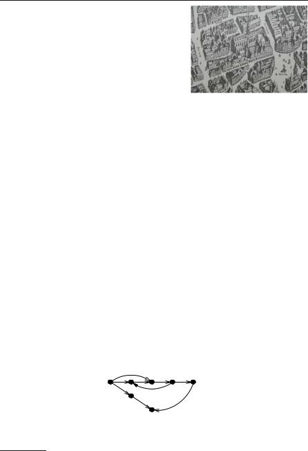
Suppose you are working in the traffic planning department of a town with a nice medieval center1. An unholy coalition of shop owners, who want more street-side parking, and the Green Party, which wants to discourage car traffic altogether, has decided to turn most streets into one-way streets. You want to avoid the worst by checking whether the current plan maintains the minimal requirement that one can still drive from every point in town to every other point.
In the language of graphs (see Sect. 2.9), the question is whether the directed graph formed by the streets is strongly connected. The same problem comes up in other applications. For example, in the case of a communication network with unidirectional channels (e.g., radio transmitters), we want to know who can communicate with whom. Bidirectional communication is possible within the strongly connected components of the graph.
We shall present a simple, efficient algorithm for computing strongly connected components (SCCs) in Sect. 9.2.2. Computing SCCs and many other fundamental problems on graphs can be reduced to systematic graph exploration, inspecting each edge exactly once. We shall present the two most important exploration strategies: breadth-first search , in Sect. 9.1, and depth-first search, in Sect. 9.2. Both strategies construct forests and partition the edges into four classes: tree edges comprising the forest, forward edges running parallel to paths of tree edges, backward edges running antiparallel to paths of tree edges, and cross edges that connect two different branches of a tree in the forest. Figure 9.1 illustrates the classification of edges.
forward |
||
s |
backward |
|
tree |
||
|
||
cross
Fig. 9.1. Graph edges classified as tree edges, forward edges, backward edges, and cross edges
1 The copper engraving above shows a part of Frankfurt around 1628 (M. Merian).
176 9 Graph Traversal
9.1 Breadth-First Search
A simple way to explore all nodes reachable from some node s is breadth-first search (BFS). BFS explores the graph layer by layer. The starting node s forms layer 0. The direct neighbors of s form layer 1. In general, all nodes that are neighbors of a node in layer i but not neighbors of nodes in layers 0 to i −1 form layer i + 1.
The algorithm in Fig. 9.2 takes a node s and constructs the BFS tree rooted at s. For each node v in the tree, the algorithm records its distance d(v) from s, and the parent node parent(v) from which v was first reached. The algorithm returns the pair (d, parent). Initially, s has been reached and all other nodes store some special valueto indicate that they have not been reached yet. Also, the depth of s is zero. The main loop of the algorithm builds the BFS tree layer by layer. We maintain two sets Q and Q ; Q contains the nodes in the current layer, and we construct the next layer in Q . The inner loops inspect all edges (u, v) leaving nodes u in the current layer Q. Whenever v has no parent pointer yet, we put it into the next layer Q and set its parent pointer and distance appropriately. Figure 9.3 gives an example of a BFS tree and the resulting backward and cross edges.
BFS has the useful feature that its tree edges define paths from s that have a minimum number of edges. For example, you could use such paths to find railway connections that minimize the number of times you have to change trains or to find paths in communication networks with a minimal number of hops. An actual path from s to a node v can be found by following the parent references from v backwards.
Exercise 9.1. Show that BFS will never classify an edge as forward, i.e., there are no edges (u, v) with d(v) > d(u) + 1.
Function bfs(s : NodeId) : (NodeArray of NodeId) ×(NodeArray of 0..n)
d = ∞, . . . , ∞ : NodeArray of NodeId |
// distance from root |
||
parent = , . . . , : NodeArray of NodeId |
|
||
d[s] := 0 |
|
|
|
parent[s] := s |
|
// self-loop signals root |
|
Q = s |
: Set of NodeId |
|
// current layer of BFS tree |
Q = |
: Set of NodeId |
|
// next layer of BFS tree |
for := 0 to ∞ while Q = do |
|
// explore layer by layer |
|
invariant Q contains all nodes with distance from s |
|
||
foreach u Q do |
|
|
|
foreach (u, v) E do |
|
// scan edges out of u |
|
|
if parent(v) = then |
|
// found an unexplored node |
|
Q := Q {v} |
|
// remember for next layer |
|
d[v] := + 1 |
|
|
|
parent(v) := u |
|
// update BFS tree |
(Q, Q ) := (Q , ) |
|
// switch to next layer |
|
return (d, parent) |
// the BFS tree is now {(v, w) : w V, v = parent(w)} |
||
Fig. 9.2. Breadth-first search starting at a node s

9.1 Breadth-First Search |
177 |
|
b |
e |
g |
tree |
|
|
|
|
s |
c |
|
|
backward s |
b |
e |
g |
f |
|
|
cross |
|
|
|
|
||
|
|
|
|
d |
|
c |
|
|
|
d |
f |
|
forward |
|
|
||
|
|
|
|
|
|
|||
|
|
|
|
|
|
|
||
0 |
1 |
2 |
3 |
|
|
|
|
|
Fig. 9.3. An example of how BFS (left) and DFS (right) classify edges into tree edges, backward edges, cross edges, and forward edges. BFS visits the nodes in the order s, b, c, d, e, f , g. DFS visits the nodes in the order s, b, e, g, f , c, d
Exercise 9.2. What can go wrong with our implementation of BFS if parent[s] is initialized to rather than s? Give an example of an erroneous computation.
Exercise 9.3. BFS trees are not necessarily unique. In particular, we have not specified in which order nodes are removed from the current layer. Give the BFS tree that is produced when d is removed before b when one performs a BFS from node s in the graph in Fig. 9.3.
Exercise 9.4 (FIFO BFS). Explain how to implement BFS using a single FIFO queue of nodes whose outgoing edges still have to be scanned. Prove that the resulting algorithm and our two-queue algorithm compute exactly the same tree if the two-queue algorithm traverses the queues in an appropriate order. Compare the FIFO version of BFS with Dijkstra’s algorithm described in Sect. 10.3, and the Jarník–Prim algorithm described in Sect. 11.2. What do they have in common? What are the main differences?
Exercise 9.5 (graph representation for BFS). Give a more detailed description of BFS. In particular, make explicit how to implement it using the adjacency array representation described in Sect. 8.2. Your algorithm should run in time O(n + m).
Exercise 9.6 (connected components). Explain how to modify BFS so that it computes a spanning forest of an undirected graph in time O(m + n). In addition, your algorithm should select a representative node r for each connected component of the graph and assign it to component[v] for each node v in the same component as r. Hint: scan all nodes s V and start BFS from any node s that it still unreached when it is scanned. Do not reset the parent array between different runs of BFS. Note that isolated nodes are simply connected components of size one.
Exercise 9.7 (transitive closure). The transitive closure G+ = (V, E+) of a graph
G = (V, E) has an edge (u, v) E+ whenever there is a path from u to v in E. Design an algorithm for computing transitive closures. Hint: run bfs(v) for each node v to find all nodes reachable from v. Try to avoid a full reinitialization of the arrays d and parent at the beginning of each call. What is the running time of your algorithm?
178 9 Graph Traversal
9.2 Depth-First Search
You may view breadth-first search as a careful, conservative strategy for systematic exploration that looks at known things before venturing into unexplored territory. In this respect, depth-first search (DFS) is the exact opposite: whenever it finds a new node, it immediately continues to explore from it. It goes back to previously explored nodes only if it runs out of options. Although DFS leads to unbalanced, strangelooking exploration trees compared with the orderly layers generated by BFS, the combination of eager exploration with the perfect memory of a computer makes DFS very useful. Figure 9.4 gives an algorithm template for DFS. We can derive specific algorithms from it by specifying the subroutines init, root, traverseTreeEdge, traverseNonTreeEdge, and backtrack.
DFS marks a node when it first discovers it; initially, all nodes are unmarked. The main loop of DFS looks for unmarked nodes s and calls DFS(s, s) to grow a tree rooted at s. The recursive call DFS(u, v) explores all edges (v, w) out of v. The argument (u, v) indicates that v was reached via the edge (u, v) into v. For root nodes s, we use the “dummy” argument (s, s). We write DFS( , v) if the specific nature of the incoming edge is irrelevant to the discussion at hand. Assume now that we are exploring edge (v, w) within the call DFS( , v).
If w has been seen before, w is already a node of the DFS forest. So (v, w) is not a tree edge, and hence we call traverseNonTreeEdge(v, w) and make no recursive call of DFS.
If w has not been seen before, (v, w) becomes a tree edge. We therefore call traverseTreeEdge(v, w), mark w, and make the recursive call DFS(v, w). When we return from this call, we explore the next edge out of v. Once all edges out of v have been explored, we call backtrack on the incoming edge (u, v) to perform any summarizing or cleanup operations needed and return.
At any point in time during the execution of DFS, there are a number of active calls. More precisely, there are nodes v1, v2, . . . vk such that we are currently exploring edges out of vk, and the active calls are DFS(v1, v1), DFS(v1, v2), . . . , DFS(vk−1, vk). In this situation, we say that the nodes v1, v2, . . . , vk are active and form the DFS recursion stack. The node vk is called the current node. We say that a node v has been reached when DFS( , v) is called, and is finished when the call DFS( , v) terminates.
Exercise 9.8. Give a nonrecursive formulation of DFS. You need to maintain a stack of active nodes and, for each active node, the set of unexplored edges.
9.2.1 DFS Numbering, Finishing Times, and Topological Sorting
DFS has numerous applications. In this section, we use it to number the nodes in two ways. As a by-product, we see how to detect cycles. We number the nodes in the order in which they are reached (array dfsNum) and in the order in which they are finished (array finishTime). We have two counters dfsPos and finishingTime, both initialized to one. When we encounter a new root or traverse a tree edge, we set the
|
9.2 |
Depth-First Search |
179 |
Depth-first search of a directed graph G = (V, E) |
|
|
|
unmark all nodes |
|
|
|
init |
|
|
|
foreach s V do |
|
|
|
if s is not marked then |
|
|
|
mark s |
|
// make s a root and grow |
|
root(s) |
// |
a new DFS tree rooted at it. |
|
DFS(s, s) |
|
|
|
Procedure DFS(u, v : NodeId) |
|
// Explore v coming from u. |
|
foreach (v, w) E do |
|
|
|
if w is marked then traverseNonTreeEdge(v, w) |
// w was reached before |
||
else traverseTreeEdge(v, w) |
|
// w was not reached before |
|
mark w |
|
|
|
DFS(v, w) |
|
|
|
backtrack(u, v) |
// return from v along the incoming edge |
||
Fig. 9.4. A template for depth-first search of a graph G = (V, E). We say that a call DFS( , v) explores v. The exploration is complete when we return from this call
dfsNum of the newly encountered node and increment dfsPos. When we backtrack from a node, we set its finishTime and increment finishingTime. We use the following subroutines:
init: |
dfsPos = 1 : 1..n; finishingTime = 1 : 1..n |
root(s): |
dfsNum[s] := dfsPos++ |
traverseTreeEdge(v, w): |
dfsNum[w] := dfsPos++ |
backtrack(u, v): |
finishTime[v] := finishingTime++ |
The ordering by dfsNum is so useful that we introduce a special notation ‘ ’ for it. For any two nodes u and v, we define
u v dfsNum[u] < dfsNum[v] .
The numberings dfsNum and finishTime encode important information about the execution of DFS, as we shall show next. We shall first show that the DFS numbers increase along any path of the DFS tree, and then show that the numberings together classify the edges according to their type.
Lemma 9.1. The nodes on the DFS recursion stack are sorted with respect to .
Proof. dfsPos is incremented after every assignment to dfsNum. Thus, when a node v becomes active by a call DFS(u, v), it has just been assigned the largest dfsNum so far.
dfsNums and finishTimes classify edges according to their type, as shown in Table 9.1. The argument is as follows. Two calls of DFS are either nested within each other, i.e., when the second call starts, the first is still active, or disjoint, i.e., when the

180 9 Graph Traversal
Table 9.1. The classification of an edge (v, w). Tree and forward edges are also easily distinguished. Tree edges lead to recursive calls, and forward edges do not
Type |
dfsNum[v] < dfsNum[w] |
finishTime[w] < FinishTime[v] |
Tree |
Yes |
Yes |
Forward |
Yes |
Yes |
Backward |
No |
No |
Cross |
No |
Yes |
|
|
|
second starts, the first is already completed. If DFS( , w) is nested in DFS( , v), the former call starts after the latter and finishes before it, i.e., dfsNum[v] < dfsNum[w] and finishTime[w] < finishTime[v]. If DFS( , w) and DFS( , v) are disjoint and the former call starts before the latter, it also ends before the latter, i.e., dfsNum[w] < dfsNum[v] and finishTime[w] < finishTime[v]. The tree edges record the nesting structure of recursive calls. When a tree edge (v, w) is explored within DFS( , v), the call DFS(v, w) is made and hence is nested within DFS( , v). Thus w has a larger DFS number and a smaller finishing time than v. A forward edge (v, w) runs parallel to a path of tree edges and hence w has a larger DFS number and a smaller finishing time than v. A backward edge (v, w) runs antiparallel to a path of tree edges, and hence w has a smaller DFS number and a larger finishing time than v. Let us look, finally, at a cross edge (v, w). Since (v, w) is not a tree, forward, or backward edge, the calls DFS( , v) and DFS( , w) cannot be nested within each other. Thus they are disjoint. So w is marked either before DFS( , v) starts or after it ends. The latter case is impossible, since, in this case, w would be unmarked when the edge (v, w) was explored, and the edge would become a tree edge. So w is marked before DFS( , v) starts and hence DFS( , w) starts and ends before DFS( , v). Thus dfsNum[w] < dfsNum[v] and finishTime[w] < finishTime[v]. The following Lemma summarizes the discussion.
Lemma 9.2. Table 9.1 shows the characterization of edge types in terms of dfsNum and finishTime.
Exercise 9.9. Modify DFS such that it labels the edges with their type. What is the type of an edge (v, w) when w is on the recursion stack when the edge is explored?
Finishing times have an interesting property for directed acyclic graphs.
Lemma 9.3. The following properties are equivalent: (i) G is an acyclic directed graph (DAG); (ii) DFS on G produces no backward edges; (iii) all edges of G go from larger to smaller finishing times.
Proof. Backward edges run antiparallel to paths of tree edges and hence create cycles. Thus DFS on an acyclic graph cannot create any backward edges. All other types of edge run from larger to smaller finishing times according to Table 9.1. Assume now that all edges run from larger to smaller finishing times. In this case the graph is clearly acyclic.
An order of the nodes of a DAG in which all edges go from left to right is called a topological sorting. By Lemma 9.3, the ordering by decreasing finishing time is a
9.2 Depth-First Search |
181 |
topological ordering. Many problems on DAGs can be solved efficiently by iterating over the nodes in a topological order. For example, in Sect. 10.2 we shall see a fast, simple algorithm for computing shortest paths in acyclic graphs.
Exercise 9.10 (topological sorting). Design a DFS-based algorithm that outputs the nodes in topological order if G is a DAG. Otherwise, it should output a cycle.
Exercise 9.11. Design a BFS-based algorithm for topological sorting.
Exercise 9.12. Show that DFS on an undirected graph does not produce any cross edges.
9.2.2 Strongly Connected Components
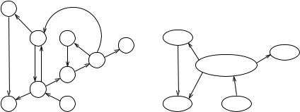
We now come back to the problem posed at the beginning of this chapter. Recall that two nodes belong to the same strongly connected component (SCC) of a graph iff they are reachable from each other. In undirected graphs, the relation “being reachable” is symmetric, and hence strongly connected components are the same as connected components. Exercise 9.6 outlines how to compute connected components using BFS, and adapting this idea to DFS is equally simple. For directed graphs, the situation is more interesting; see Fig. 9.5 for an example. We shall show that an extension of DFS computes the strongly connected components of a digraph G in linear time O(n + m). More precisely, the algorithm will output an array component indexed by nodes such that component[v] = component[w] iff v and w belong to the same SCC. Alternatively, it could output the node set of each SCC.
Exercise 9.13. Show that the node sets of distinct SCCs are disjoint. Hint: assume that SCCs C and D have a common node v. Show that any node in C can reach any node in D and vice versa.
e
d |
h |
e |
i
i
g
c, d, f , g, h
f
c
a |
b |
a |
b |
Fig. 9.5. A digraph G and the corresponding shrunken graph Gs. The SCCs of G have node sets {a}, {b}, {c, d, f , g, h}, {e}, and {i}
182 |
9 |
Graph Traversal |
|
|
|
|
|
e |
|
|
|
|
|
|
|
|
|
e |
|
|
|
|
d |
h |
|
|
fgh |
|
|
|
|
|
||
|
|
|
|
|
cd |
|
|
|
|
|
g |
|
|
|
|
|
f |
a |
b |
|
|
|
c |
|
|
|
|
|
a |
|
b |
open nodes |
b c d |
f g h |
|
|
|
|
representatives b c |
f |
|
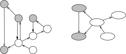
Fig. 9.6. A snapshot of DFS on the graph of Fig. 9.5 and the corresponding shrunken graph. The first DFS was started at node a and a second DFS was started at node b, the current node is g, and the recursion stack contains b, c, f , g. The edges (g, i) and (g, d) have not been explored yet. Edges (h, f ) and (d, c) are back edges, (e, a) is a cross edge, and all other edges are tree edges. Finished nodes and closed components are shaded. There are closed components {a} and {e} and open components {b}, {c, d}, and { f , g, h}. The open components form a path in the shrunken graph with the current node g belonging to the last component. The representatives of the open components are the nodes b, c, and f , respectively. DFS has reached the open nodes in the order b, c, d, f , g, h. The representatives partition the sequence of open nodes into the SCCs of Gc
The idea underlying the algorithm is simple. We imagine that the edges of G are added one by one to an initially edgeless graph. We use Gc = (V, Ec) to denote the current graph, and keep track of how the SCCs of Gc evolve as edges are added. Initially, there are no edges and each node forms an SCC of its own. For the addition step, it is helpful to introduce the notion of a shrunken graph. We use Gsc to denote the shrunken graph corresponding to Gc. The nodes of Gsc are the SCCs of Gc. If C and D are distinct SCCs of Gc, we have an edge (C, D) in Gsc iff there are nodes u C and v D where (u, v) is an edge of Gc. Figure 9.5 shows an example.
Lemma 9.4. The shrunken graph Gsc is acyclic.
Proof. Assume otherwise, and let C1,C2, . . . ,Ck−1,Ck with Ck = C1 be a cycle in Gsc. Recall that the Ci are SCCs of Gc. By the definition of Gsc, Gc contains an edge (vi, wi+1) with vi Ci and wi+1 Ci+1 for 0 ≤ i < k. Define vk = v1. Since Ci is strongly connected, Gc contains a path from wi+1 to vi+1, 0 ≤ i < k.Thus all the vi’s belong to the same SCC, a contradiction.
How do the SCCs of Gc and Gsc change when we add an edge e to Gc? There are three cases to consider. (1) Both endpoints of e belong to the same SCC of Gc. The shrunken graph and the SCCs do not change. (2) e connects nodes in different SCCs but does not close a cycle. The SCCs do not change, and an edge is added to the shrunken graph. (3) e connects nodes in different SCCs and closes one or more