

Algorithms and data structures
.pdf204 10 Shortest Paths
|
Case i<K |
|
|
Case |
i=K |
|
|
||||
|
|
i |
0 |
|
|
j |
|
|
h 0 |
||
mino |
α |
0 |
|
|
|
α |
0 |
|
|
|
|
min |
|
|
|
|
|
|
|
|
|
|
|
α |
1 |
|
|
α |
1 |
β |
|
0 |
|
||
x |
|
|
|
|
|
|
|
|
|
|
|
α |
1 |
|
|
α |
1 |
β |
|
1 |
|
||
Fig. 10.8. The structure of the keys relevant to the proof of Lemma 10.7. In the proof, it is shown that β starts with j − K zeros
Proof. Observe Þrst that the case x = min is easy, since msd(x, x) = −1 < i. For the nontrivial case x =min, we distinguish the subcases i < K and i = K. Let mino be the old value of min. Figure 10.8 shows the structure of the relevant keys.
Case i < K. The most signiÞcant distinguishing index of mino and any x B[i] is i, i.e., mino has a zero in bit position i, and all x B[i] have a one in bit position i. They agree in all positions with an index larger than i. Thus the most signiÞcant distinguishing index for min and x is smaller than i.
Case i = K. Consider any x B[K]. Let j = msd(mino, min). Then j ≥ K, since min B[K]. Let h = msd(min, x). We want to show that h < K. Let α comprise the bits in positions larger than j in mino, and let A be the number obtained from mino by setting the bits in positions 0 to j to zero. Then α followed by j + 1 zeros is the binary
representation of A. Since the j-th bit of mino is zero and that of min is one, we have mino < A + 2 j and A + 2 j ≤ min. Also, x ≤ mino +C < A + 2 j +C ≤ A + 2 j + 2K . So
A + 2 j ≤ min ≤ x < A + 2 j + 2K ,
and hence the binary representations of min and x consist of α followed by a 1, followed by j − K zeros, followed by some bit string of length K. Thus min and x agree in all bits with index K or larger, and hence h < K.
In order to aid intuition, we give a second proof for the case i = K. We Þrst observe that the binary representation of min starts with α followed by a one. We next observe that x can be obtained from mino by adding some K-bit number. Since min ≤ x, the Þnal carry in this addition must run into position j. Otherwise, the j-th bit of x would be zero and hence x < min. Since mino has a zero in position j, the carry stops at position j. We conclude that the binary representation of x is equal to α followed by a 1, followed by j − K zeros, followed by some K-bit string. Since min ≤ x, the j −K zeros must also be present in the binary representation of min.
*Exercise 10.12. Radix heaps can also be based on number representations with base b for any b ≥ 2. In this situation we have buckets B[i, j] for i = −1, 0, 1, . . . , K and 0 ≤ j ≤ b, where K = 1 + logC/ log b . An unscanned reached node x is stored in bucket B[i, j] if msd(min, d[x]) = i and the i-th digit of d[x] is equal to j. We also store, for each i, the number of nodes contained in the buckets jB[i, j]. Discuss the implementation of the priority queue operations and show that a shortest-path
10.5 Monotone Integer Priority Queues |
205 |
algorithm with running time O(m + n(b + logC/ log b)) results. What is the optimal choice of b?
If the edge costs are random integers in the range 0..C, a small change to DijkstraÕs algorithm with radix heaps guarantees linear running time [139, 76]. For every node v, let cinmin(v) denote the minimum cost of an incoming edge. We divide Q into two parts, a set F which contains unscanned nodes whose tentative-distance label is known to be equal to their exact distance from s, and a part B which contains all other reached unscanned nodes. B is organized as a radix heap. We also maintain a value min. We scan nodes as follows.
When F is nonempty, an arbitrary node in F is removed and the outgoing edges are relaxed. When F is empty, the minimum node is selected from B and min is set to its distance label. When a node is selected from B, the nodes in the Þrst nonempty
bucket B[i] are redistributed if i ≥ 0. There is a small change in the redistribution
process. When a node v is to be moved, and d[v] ≤ min + cinmin(v), we move v to F. Observe that any future relaxation of an edge into v cannot decrease d[v], and hence
d[v] is known to be exact at this point.
We call this algorithm ALD (average-case linear Dijkstra). The algorithm ALD is correct, since it is still true that d[v] = μ (v) when v is scanned. For nodes removed from F, this was argued in the previous paragraph, and for nodes removed from B, this follows from the fact that they have the smallest tentative distance among all unscanned reached nodes.
Theorem 10.8. Let G be an arbitrary graph and let c be a random function from E to 0..C. The algorithm ALD then solves the single-source problem in expected time
O(m + n).
Proof. We still need to argue the bound on the running time. To do this, we modify the amortized analysis of plain radix heaps. As before, nodes start out in B[K]. When
a node v has been moved to a new bucket but not yet to F, d[v] > min + cinmin(v), and hence v is moved to a bucket B[i] with i ≥ log cinmin(v). Hence, it sufÞces if insert pays K − log cinmin(v) + 1 tokens into the account for node v in order to cover all costs due to decreaseKey and deleteMin operations operating on v. Summing over all nodes,
we obtain a total payment of
∑(K − log cinmin(v) + 1) = n + ∑(K − log cinmin(v)) .
v |
v |
We need to estimate this sum. For each vertex, we have one incoming edge contributing to this sum. We therefore bound the sum from above if we sum over all edges,
i.e.,
∑(K − log cinmin(v)) ≤ ∑(K − log c(e)) .
v |
e |
K −log c(e) is the number of leading zeros in the binary representation of c(e) when written as a K-bit number. Our edge costs are uniform random numbers in 0..C, and K = 1 + logC . Thus prob(K −log c(e) = i) = 2−i. Using (A.14), we conclude that
206 10 Shortest Paths
E ∑(k − log c(e)) |
= ∑ ∑ i2−i = O(m) . |
e |
e i≥0 |
Thus the total expected cost of the deleteMin and decreaseKey operations is O(m + n). The time spent outside these operations is also O(m + n).
It is a little odd that the maximum edge cost C appears in the premise but not in the conclusion of Theorem 10.8. Indeed, it can be shown that a similar result holds for random real-valued edge costs.
**Exercise 10.13. Explain how to adapt the algorithm ALD to the case where c is a random function from E to the real interval (0, 1]. The expected time should still be O(m + n). What assumptions do you need about the representation of edge costs and about the machine instructions available? Hint: you may Þrst want to solve Exercise 10.11. The narrowest bucket should have a width of mine E c(e). Subsequent buckets have geometrically growing widths.
10.6 Arbitrary Edge Costs (Bellman–Ford Algorithm)
For acyclic graphs and for nonnegative edge costs, we got away with m edge relaxations. For arbitrary edge costs, no such result is known. However, it is easy to guarantee the correctness criterion of Lemma 10.3 using O(n · m) edge relaxations: the BellmanÐFord algorithm [18, 63] given in Fig. 10.9 performs n − 1 rounds. In each round, it relaxes all edges. Since simple paths consist of at most n − 1 edges, every shortest path is a subsequence of this sequence of relaxations. Thus, after the relaxations are completed, we have d[v] = μ (v) for all v with −∞ < d[v] < ∞, by Lemma 10.3. Moreover, parent encodes the shortest paths to these nodes. Nodes v unreachable from s will still have d[v] = ∞, as desired.
It is not so obvious how to Þnd the nodes v with μ (v) = −∞. Consider any edge e = (u, v) with d[u] + c(e) < d[v] after the relaxations are completed. We can set d[v] := −∞ because if there were a shortest path from s to v, we would have found it by now and relaxing e would not lead to shorter distances anymore. We can now also set d[w] = −∞ for all nodes w reachable from v. The pseudocode implements this approach using a recursive function infect(v). It sets the d-value of v and all nodes reachable from it to −∞. If infect reaches a node w that already has d[w] = −∞, it breaks the recursion because previous executions of infect have already explored all nodes reachable from w. If d[v] is not set to −∞ during postprocessing, we have d[x] + c(e) ≥ d[y] for any edge e = (x, y) on any path p from s to v. Thus d[s] + c( p) ≥ d[v] for any path p from s to v, and hence d[v] ≤ μ (v). We conclude that d[v] = μ (v).
Exercise 10.14. Show that the postprocessing runs in time O(m). Hint: relate infect to DFS.
Exercise 10.15. Someone proposes an alternative postprocessing algorithm: set d[v] to −∞ for all nodes v for which following parents does not lead to s. Give an example where this method overlooks a node with μ (v) = −∞.
10.7 All-Pairs Shortest Paths and Node Potentials |
207 |
|
Function BellmanFord(s : NodeId) : NodeArray×NodeArray |
|
|
d = ∞, . . . , ∞ : NodeArray of R {−∞, ∞} |
// distance from root |
|
parent = , . . . , : NodeArray of NodeId |
|
|
d[s] := 0; parent[s] := s |
// self-loop signals root |
|
for i := 1 to n − 1 do |
|
|
forall e E do relax(e) |
// round i |
|
forall e = (u, v) E do |
// postprocessing |
|
if d[u] + c(e) < d[v] then infect(v) |
|
|
return (d, parent) |
|
|
Procedure infect(v) if d[v] > −∞ then
d[v] := −∞
foreach (v, w) E do infect(w)
Fig. 10.9. The BellmanÐFord algorithm for shortest paths in arbitrary graphs
Exercise 10.16 (arbitrage). Consider a set of currencies C with an exchange rate of ri j between currencies i and j (you obtain ri j units of currency j for one unit of currency i). A currency arbitrage is possible if there is a sequence of elementary currency exchange actions (transactions) that starts with one unit of a currency and ends with more than one unit of the same currency. (a) Show how to Þnd out whether a matrix of exchange rates admits currency arbitrage. Hint: log(xy) = log x+ log y. (b) ReÞne your algorithm so that it outputs a sequence of exchange steps that maximizes the average proÞt per transaction.
Section 10.10 outlines further reÞnements of the BellmanÐFord algorithm that are necessary for good performance in practice.
10.7 All-Pairs Shortest Paths and Node Potentials
The all-pairs problem is tantamount to n single-source problems and hence can be solved in time O n2m . A considerable improvement is possible. We shall show that it sufÞces to solve one general single-source problem plus n single-source problems with nonnegative edge costs. In this way, we obtain a running time of O(nm + n(m + n logn)) = O nm + n2 log n . We need the concept of node potentials.
A (node) potential function assigns a number pot(v) to each node v. For an edge e = (v, w), we deÞne its reduced cost cø(e) as
cø(e) = pot(v) + c(e) − pot(w) .
Lemma 10.9. Let p and q be paths from v to w. Then cø( p) = pot(v) + c(p) −pot(w) and cø( p) ≤ cø(q) iff c( p) ≤ c(q). In particular, the shortest paths with respect to cø are the same as those with respect to c.
208 |
10 Shortest Paths |
|
All-Pairs Shortest Paths in the Absence of Negative Cycles |
|
|
add a new node s and zero length edges (s, v) for all v |
// no new cycles, time O(m) |
|
compute μ (v) for all v with BellmanÐFord |
// time O(nm) |
|
set pot(v) = μ (v) and compute reduced costs cø(e) for e E |
// time O(m) |
|
forall nodes x do |
// time O(n(m + n log n)) |
|
|
|
ø |
|
use DijkstraÕs algorithm to compute the reduced shortest-path distances μ (x, v) |
|
|
using source x and the reduced edge costs cø |
|
// translate distances back to original cost function |
// time O(m) |
|
|
ø |
// use Lemma 10.9 |
forall e = (v, w) V ×V do μ (v, w) := μ (v, w) + pot(w) − pot(v) |
||
Fig. 10.10. Algorithm for all-pairs shortest paths in the absence of negative cycles
Proof. The second and the third claim follow from the Þrst. For the Þrst claim, let p = e0, . . . , ek−1 , where ei = (vi, vi+1), v = v0, and w = vk. Then
k−1 |
= ∑ (pot(vi) + c(ei) − pot(vi+1)) |
|
cø(p) = ∑ cø(ei) |
|
|
i=0 |
0≤i<k |
|
= pot(v0) + |
∑ c(ei) − pot(vk) = pot(v0) + c(p) − pot(vk) . |
|
|
0≤i<k |
|
Exercise 10.17. Node potentials can be used to generate graphs with negative edge costs but no negative cycles: generate a (random) graph, assign to every edge e a (random) nonnegative cost c(e), assign to every node v a (random) potential pot(v), and set the cost of e = (u, v) to cø(e) = pot(u) + c(e) − pot(v). Show that this rule does not generate negative cycles.
Lemma 10.10. Assume that reached from s. Let pot(v) = edge costs are nonnegative.
G has no negative cycles and that all nodes can be μ (v) for v V . With these node potentials, the reduced
Proof. Since all nodes are reachable from s and since there are no negative cycles, μ (v) R for all v. Thus the reduced costs are well deÞned. Consider an arbitrary edge e = (v, w). We have μ (v) + c(e) ≥ μ (w), and thus cø(e) = μ (v) + c(e) −μ (w) ≥ 0.
Theorem 10.11. The all-pairs shortest-path problem for a graph without negative cycles can be solved in time O nm + n2 log n .
Proof. The algorithm is shown in Fig. 10.10. We add an auxiliary node s and zerocost edges (s, v) for all nodes of the graph. This does not create negative cycles and does not change μ (v, w) for any of the existing nodes. Then we solve the singlesource problem for the source s, and set pot(v) = μ (v) for all v. Next we compute the reduced costs and then solve the single-source problem for each node x by means of DijkstraÕs algorithm. Finally, we translate the computed distances back to the original cost function. The computation of the potentials takes time O(nm), and the n shortestpath calculations take time O(n(m + n log n)). The preprocessing and postprocessing take linear time.
10.8 Shortest-Path Queries |
209 |
The assumption that G has no negative cycles can be removed [133].
Exercise 10.18. The diameter D of a graph G is deÞned as the largest distance between any two of its nodes. We can easily compute it using an all-pairs computation. Now we want to consider ways to approximate the diameter of a strongly
connected graph using a constant number of single-source computations. (a) For any starting node s, let D (s) := maxu V μ (u). Show that D (s) ≤ D ≤ 2D (s) for undirected graphs. Also, show that no such relation holds for directed graphs. Let D (s) := maxu V μ (u, s). Show that max(D (s), D (s)) ≤ D ≤ D (s) + D (s) for both undirected and directed graphs. (b) How should a graph be represented to support
both forward and backward search? (c) Can you improve the approximation by considering more than one node s?
10.8 Shortest-Path Queries
We are often interested in the shortest path from a speciÞc source node s to a speciÞc target node t; route planning in a trafÞc network is one such scenario. We shall explain some techniques for solving such shortest-path queries efÞciently and argue for their usefulness for the route-planning application.
We start with a technique called early stopping. We run DijkstraÕs algorithm to Þnd shortest paths starting at s. We stop the search as soon as t is removed from the priority queue, because at this point in time the shortest path to t is known. This helps except in the unfortunate case where t is the node farthest from s. On average, early stopping saves a factor of two in scanned nodes in any application. In practical route planning, early stopping saves much more because modern car navigation systems have a map of an entire continent but are mostly used for distances up to a few hundred kilometers.
Another simple and general heuristic is bidirectional search, from s forward and from t backward until the search frontiers meet. More precisely, we run two copies of DijkstraÕs algorithm side by side, one starting from s and one starting from t (and running on the reversed graph). The two copies have their own queues, say Qs and Qt , respectively. We grow the search regions at about the same speed, for example by removing a node from Qs if min Qs ≤ min Qt and a node from Qt otherwise.
It is tempting to stop the search once the Þrst node u has been removed from both queues, and to claim that μ (t) = μ (s, u) + μ (u, t). Observe that execution of DijkstraÕs algorithm on the reversed graph with a starting node t determines μ (u, t). This is not quite correct, but almost so.
Exercise 10.19. Give an example where u is not on the shortest path from s to t.
However, we have collected enough information once some node u has been removed from both queues. Let ds and dt denote the tentative-distance labels at the time of termination in the runs with source s and source t, respectively. We show that μ (t) < μ (s, u) + μ (u, t) implies the existence of a node v Qs with μ (t) = ds[v] + dt [v].

210 10 Shortest Paths
Let p = s = v0, . . . , vi, vi+1, . . . , vk = t be a shortest path from s to t. Let i be maximal such that vi has been removed from Qs. Then ds[vi+1] = μ (s, vi+1) and vi+1 Qs when the search stops. Also, μ (s, u) ≤ μ (s, vi+1), since u has already been removed from Qs, but vi+1 has not. Next, observe that
μ (s, vi+1) + μ (vi+1, t) = c( p) < μ (s, u) + μ (u, t) , since p is a shortest path from s to t. By subtracting μ (s, vi+1), we obtain
μ (vi+1, t) < μ (s, u) − μ (s, vi+1) +μ (u, t) ≤ μ (u, t)
≤0
and hence, since u has been scanned from t, vi+1 must also have been scanned from t, i.e., dt [vi+1] = μ (vi+1, t) when the search stops. So we can determine the shortest distance from s to t by inspecting not only the Þrst node removed from both queues, but also all nodes in, say, Qs. We iterate over all such nodes v and determine the minimum value of ds[v] + dt [v].
DijkstraÕs algorithm scans nodes in order of increasing distance from the source. In other words, it grows a circle centered on the source node. The circle is deÞned by the shortest-path metric in the graph. In the route-planning application for a road network, we may also consider geometric circles centered on the source and argue that shortest-path circles and geometric circles are about the same. We can then estimate the speedup obtained by bidirectional search using the following heuristic argument: a circle of a certain diameter has twice the area of two circles of half the diameter. We could thus hope that bidirectional search will save a factor of two compared with unidirectional search.
Exercise 10.20 (bidirectional search). (a) Consider bidirectional search in a grid graph with unit edge weights. How much does it save over unidirectional search? (*b) Try to Þnd a family of graphs where bidirectional search visits exponentially fewer nodes on average than does unidirectional search. Hint: consider random graphs or hypercubes. (c) Give an example where bidirectional search in a real road network takes longer than unidirectional search. Hint: consider a densely inhabitated city with sparsely populated surroundings. (d) Design a strategy for switching between forward and backward search such that bidirectional search will never inspect more than twice as many nodes as unidirectional search.
We shall next describe two techniques that are more complex and less generally applicable: however, if they are applicable, they usually result in larger savings. Both techniques mimic human behavior in route planning.
10.8.1 Goal-Directed Search
The idea is to bias the search space such that DijkstraÕs algorithm does not grow a disk but a region protruding toward the target; see Fig. 10.11. Assume we know a function f : V → R that estimates the distance to the target, i.e., f (v) estimates
10.8 Shortest-Path Queries |
211 |
μ (v, t) for all nodes v. We use the estimates to modify the distance function. For each e = (u, v), let4 cø(e) = c(e) + f (v) − f (u). We run DijkstraÕs algorithm with
the modiÞed distance function. We know already that node potentials do not change shortest paths, and hence correctness is preserved. Tentative distances are related via dø[v] = d[v] + f (v) − f (s). An alternative view of this modiÞcation is that we run DijkstraÕs algorithm with the original distance function but remove the node with
minimal value d[v] + f (v) from the queue. The algorithm just described is known as
A -search.
s |
t |
s |
t |
Fig. 10.11. The standard Dijkstra search grows a circular region centered on the source; goaldirected search grows a region protruding toward the target
Before we state requirements on the estimate f , let us see one speciÞc example. Assume, in a thought experiment, that f (v) = μ (v, t). Then cø(e) = c(e) + μ (v, t) − μ (u, t) and hence edges on a shortest path from s to t have a modiÞed cost equal to zero and all other edges have a positive cost. Thus DijkstraÕs algorithm only follows shortest paths, without looking left or right.
The function f must have certain properties to be useful. First, we want the modiÞed distances to be nonnegative. So, we need c(e) + f (v) ≥ f (u) for all edges e = (u, v). In other words, our estimate of the distance from u should be at most our estimate of the distance from v plus the cost of going from u to v. This property is called consistency of estimates. We also want to be able to stop the search when t is removed from the queue. This works if f is a lower bound on the distance to the target, i.e., f (v) ≤ μ (v, t) for all v V . Then f (t) = 0. Consider the point in time when t is removed from the queue, and let p be any path from s to t. If all edges of p have been relaxed at termination, d[t] ≤ c( p). If not all edges of p have been relaxed at termination, there is a node v on p that is contained in the queue at termination. Then d(t) + f (t) ≤ d(v) + f (v), since t was removed from the queue but v was not, and hence
d[t] = d[t] + f (t) ≤ d[v] + f (v) ≤ d[v] + μ (v, t) ≤ c( p) .
In either case, we have d[t] ≤ c( p), and hence the shortest distance from s to t is known as soon as t is removed from the queue.
What is a good heuristic function for route planning in a road network? Route planners often give a choice between shortest and fastest connections. In the case
4In Sect. 10.7, we added the potential of the source and subtracted the potential of the target.
We do exactly the opposite now. The reason for changing the sign convention is that in Lemma 10.10, we used μ (s, v) as the node potential. Now, f estimates μ (v, t).
212 10 Shortest Paths
of shortest paths, a feasible lower bound f (v) is the straight-line distance between v and t. Speedups by a factor of roughly four are reported in the literature. For fastest paths, we may use the geometric distance divided by the speed assumed for the best kind of road. This estimate is extremely optimistic, since targets are frequently in the center of a town, and hence no good speedups have been reported. More sophisticated methods for computing lower bounds are known; we refer the reader to [77] for a thorough discussion.
10.8.2 Hierarchy
Road networks usually contain a hierarchy of roads: throughways, state roads, county roads, city roads, and so on. Average speeds are usually higher on roads of higher status, and therefore the fastest routes frequently follow the pattern that one starts on a road of low status, changes several times to roads of higher status, drives the largest fraction of the path on a road of high status, and Þnally changes down to lower-status roads near the target. A heuristic approach may therefore restrict the search to high-status roads except for suitably chosen neighborhoods of the source and target. Observe, however, that the choice of neighborhood is nonobvious, and that this heuristic sacriÞces optimality. You may be able to think of an example from your driving experience where shortcuts over small roads are required even far away from the source and target. Exactness can be combined with the idea of hierarchies if the hierarchy is deÞned algorithmically and is not taken from the ofÞcial classiÞcation of roads. We now outline one such approach [165], called highway hierarchies. It Þrst deÞnes a notion of locality, say anything within a distance of 10 km from either the source or the target. An edge (u, v) E is a highway edge with respect to this notion of locality if there is a source node s and a target node t such that (u, v) is on the fastest path from s to t, v is not within the local search radius of s, and u is not within the local (backward) search radius of t. The resulting network is called the highway network. It usually has many vertices of degree two. Think of a fast road to which a slow road connects. The slow road is not used on any fastest path outside the local region of a nearby source or nearby target, and hence will not be in the highway network. Thus the intersection will have degree three in the original road network, but will have degree two in the highway network. Two edges joined by a degree-two node may be collapsed into a single edge. In this way, the core of the highway network is determined. Iterating this procedure of Þnding a highway network and contracting degree-two nodes leads to a hierarchy of roads. For example, in the case of the road networks of Europe and North America, a hierarchy of up to ten levels resulted. Route planning using the resulting highway hierarchy can be several thousand times faster than DijkstraÕs algorithm.
10.8.3 Transit Node Routing
Using another observation from daily life, we can get even faster [15]. When you drive to somewhere Òfar awayÓ, you will leave your current location via one of only a few ÒimportantÓ trafÞc junctions. It turns out that in real-world road networks about
10.9 Implementation Notes |
213 |
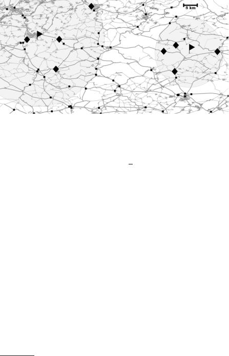
Fig. 10.12. Finding the optimal travel time between two points (the ßags) somewhere between SaarbrŸcken and Karlsruhe amounts to retrieving the 2 × 4 access nodes (diamonds), performing 16 table lookups between all pairs of access nodes, and checking that the two disks deÞning the locality filter do not overlap. The small squares indicate further transit nodes
√
99% of all quickest paths go through about O( n) important transit nodes that can be automatically selected, for example using highway hierarchies. Moreover, for each particular source or target node, all long-distance connections go through one of about ten of these transit nodes Ð the access nodes. During preprocessing, we compute a complete distance table between the transit nodes, and the distances from all nodes to their access nodes. Now, suppose we have a way to tell that a source s and a target t are sufÞciently far apart.5 There must then be access nodes as and at such that μ (t) = μ (as) + μ (as, at ) + μ (at , t). All these distances have been precomputed and there are only about ten candidates for as and for at , respectively, i.e., we need (only) about 100 accesses to the distance table. This can be more than 1 000 000 times faster than DijkstraÕs algorithm. Local queries can be answered using some other technique that will proÞt from the closeness of the source and target. We can also cover local queries using additional precomputed tables with more local information. Figure 10.12 from [15] gives an example.
10.9 Implementation Notes
Shortest-path algorithms work over the set of extended reals R {+∞, −∞}. We may ignore −∞, since it is needed only in the presence of negative cycles and, even there, it is needed only for the output; see Sect. 10.6. We can also get rid of +∞ by noting that parent(v) = iff d[v] = +∞, i.e., when parent(v) = , we assume that d[v] = +∞ and ignore the number stored in d[v].
5 We may need additional preprocessing to decide this.