

Algorithms and data structures
.pdf7.6 Implementation Notes |
163 |
element comparisons can be minimized by choosing a as a large power of two and b = 2a. Since the number of pointer dereferences is proportional to the height of the tree (see Exercise 7.4), large values of a are also good for this measure. Taking this reasoning to the extreme, we would obtain the best performance for a ≥ n, i.e., a single sorted array. This is not astonishing. We have concentrated on searches, and static data structures are best if updates are neglected.
Insertions and deletions have an amortized cost of one locate plus a constant number of node reorganizations (split, balance, or fuse) with cost O(b) each. We obtain a logarithmic amortized cost for update operations if b = O(log n). A more detailed analysis (see Exercise 7.16) would reveal that increasing b beyond 2a makes split and fuse operations less frequent and thus saves expensive calls to the memory manager associated with them. However, this measure has a slightly negative effect on the performance of locate and it clearly increases space consumption. Hence, b should remain close to 2a.
Finally, let us take a closer look at the role of cache faults. A cache of size M can hold Θ(M/b) nodes. These are most likely to be the frequently accessed nodes close to the root. To a first approximation, the top loga(M/b) levels of the tree are stored in the cache. Below this level, every pointer dereference is associated with a cache fault, i.e., we will have about loga(bn/Θ(M)) cache faults in each locate operation. Since the cache blocks of processor caches start at addresses that are a multiple of the block size, it makes sense to align the starting addresses of search tree nodes with a cache block, i.e., to make sure that they also start at an address that is a multiple of the block size. Note that (a, b)-trees might well be more efficient than binary search for large data sets because we may save a factor of log a in cache faults.
Very large search trees are stored on disks. Under the name B-trees [16], (a, b)- trees are the workhorse of the indexing data structures in databases. In that case, internal nodes have a size of several kilobytes. Furthermore, the items of the linked list are also replaced by entire data blocks that store between a and b elements, for appropriate values of a and b (see also Exercise 3.20). These leaf blocks will then also be subject to splitting, balancing, and fusing operations. For example, assume that we have a = 210, the internal memory is large enough (a few megabytes) to cache the root and its children, and the data blocks store between 16 and 32 Kbyte of data. Then two disk accesses are sufficient to locate any element in a sorted sequence that takes 16 Gbyte of storage. Since putting elements into leaf blocks dramatically decreases the total space needed for the internal nodes and makes it possible to perform very fast range queries, this measure can also be useful for a cache-efficient internalmemory implementation. However, note that update operations may now move an element in memory and thus will invalidate element handles stored outside the data structure. There are many more tricks for implementing (external-memory) (a, b)- trees. We refer the reader to [79] and [141, Chaps. 2 and 14] for overviews. A good free implementation of B-trees is available in STXXL [48].
From the augmentations discussed in Sect. 7.5 and the implementation tradeoffs discussed here, it becomes evident that the optimal implementation of sorted sequences does not exist but depends on the hardware and the operation mix relevant to the actual application. We believe that (a, b)-trees with b = 2k = 2a = O(log n), aug-

164 7 Sorted Sequences
mented with parent pointers and a doubly linked list of leaves, are a sorted-sequence data structure that supports a wide range of operations efficiently.
Exercise 7.26. What choice of a and b for an (a, b)-tree guarantees that the number of I/O operations required for insert, remove, or locate is O(logB(n/M))? How many I/O operations are needed to build an n-element (a, b)-tree using the external sorting algorithm described in Sect. 5.7 as a subroutine? Compare this with the number of I/Os needed for building the tree naively using insertions. For example, try M = 229 bytes, B = 218 bytes7, n = 232, and elements that have 8-byte keys and 8 bytes of associated information.
7.6.1 C++
The STL has four container classes set, map, multiset, and multimap for sorted sequences. The prefix multi means that there may be several elements with the same key. Maps offer the interface of an associative array (see also Chap. 4). For example, someMap[k] := x inserts or updates the element with key k and sets the associated information to x.
The most widespread implementation of sorted sequences in STL uses a variant of red–black trees with parent pointers, where elements are stored in all nodes rather than only in the leaves. None of the STL data types supports efficient splitting or concatenation of sorted sequences.
LEDA [118] offers a powerful interface sortseq that supports all important operations on sorted sequences, including finger search, concatenation, and splitting. Using an implementation parameter, there is a choice between (a, b)-trees, red–black trees, randomized search trees, weight-balanced trees, and skip lists.
7.6.2 Java
The Java library java.util offers the interface classes SortedMap and SortedSet, which correspond to the STL classes set and map, respectively. The corresponding implementation classes TreeMap and TreeSet are based on red–black trees.
7.7 Historical Notes and Further Findings
There is an entire zoo of sorted sequence data structures. Just about any of them will do if you just want to support insert, remove, and locate in logarithmic time. Performance differences for the basic operations are often more dependent on implementation details than on the fundamental properties of the underlying data structures. The differences show up in the additional operations.
7We are making a slight oversimplification here, since in practice one will use much smaller block sizes for organizing the tree than for sorting.
7.7 Historical Notes and Further Findings |
165 |
The first sorted-sequence data structure to support insert, remove, and locate in logarithmic time was AVL trees [4]. AVL trees are binary search trees which maintain the invariant that the heights of the subtrees of a node differ by one at the most. Since this is a strong balancing condition, locate is probably a little faster than in most competitors. On the other hand, AVL trees do not have constant amortized update costs. Another small disadvantage is that storing the heights of subtrees costs additional space. In comparison, red–black trees have slightly higher costs for locate, but they have faster updates and the single color bit can often be squeezed in somewhere. For example, pointers to items will always store even addresses, so that their least significant bit could be diverted to storing color information.
(2, 3)-trees were introduced in [6]. The generalization to (a, b)-trees and the amortized analysis of Sect. 3.3 come from [95]. There, it was also shown that the total number of splitting and fusing operations at the nodes of any given height decreases exponentially with the height.
Splay trees [183] and some variants of randomized search trees [176] work even without any additional information besides one key and two successor pointers. A more interesting advantage of these data structures is their adaptability to nonuniform access frequencies. If an element e is accessed with probability p, these search trees will be reshaped over time to allow an access to e in a time O(log(1/ p)). This can be shown to be asymptotically optimal for any comparison-based data structure. However, this property leads to improved running time only for quite skewed access patterns because of the large constants.
Weight-balanced trees [150] balance the size of the subtrees instead of the height. They have the advantage that a node of weight w (= number of leaves of its subtree) is only rebalanced after Ω(w) insertions or deletions have passed through it [26].
There are so many search tree data structures for sorted sequences that these two terms are sometimes used as synonyms. However, there are also some equally interesting data structures for sorted sequences that are not based on search trees. Sorted arrays are a simple static data structure. Sparse tables [97] are an elegant way to make sorted arrays dynamic. The idea is to accept some empty cells to make insertion easier. Reference [19] extended sparse tables to a data structure which is asymptotically optimal in an amortized sense. Moreover, this data structure is a crucial ingredient for a sorted-sequence data structure [19] that is cache-oblivious [69], i.e., it is cacheefficient on any two levels of a memory hierarchy without even knowing the size of caches and cache blocks. The other ingredient is oblivious static search trees [69]; these are perfectly balanced binary search trees stored in an array such that any search path will exhibit good locality in any cache. We describe here the van Emde Boas layout used for this purpose, for the case where there are n = 22k leaves for some integer k. We store the top 2k−1 levels of the tree at the beginning of the array. After that, we store the 2k−1 subtrees of depth 2k−1, allocating consecutive blocks of memory for them. We recursively allocate the resulting 1 + 2k−1 subtrees of depth 2k−1. Static cache-oblivious search trees are practical in the sense that they can outperform binary search in a sorted array.
Skip lists [159] are based on another very simple idea. The starting point is a sorted linked list . The tedious task of scanning during locate can be accelerated
166 7 Sorted Sequences
by producing a shorter list that contains only some of the elements in . If corresponding elements of and are linked, it suffices to scan and only descend to when approaching the searched element. This idea can be iterated by building shorter and shorter lists until only a single element remains in the highest-level list. This data structure supports all important operations efficiently in an expected sense. Randomness comes in because the decision about which elements to lift to a higher-level list is made randomly. Skip lists are particularly well suited for supporting finger search.
Yet another family of sorted-sequence data structures comes into play when we no longer consider keys as atomic objects. If keys are numbers given in binary representation, we can obtain faster data structures using ideas similar to the fast integer-sorting algorithms described in Sect. 5.6. For example, we can obtain sorted sequences with w-bit integer keys that support all operations in time O(log w) [198, 129]. At least for 32-bit keys, these ideas bring a considerable speedup in practice [47]. Not astonishingly, string keys are also important. For example, suppose we want to adapt (a, b)-trees to use variable-length strings as keys. If we want to keep a fixed size for node objects, we have to relax the condition on the minimal degree of a node. Two ideas can be used to avoid storing long string keys in many nodes. Common prefixes of keys need to be stored only once, often in the parent nodes. Furthermore, it suffices to store the distinguishing prefixes of keys in inner nodes, i.e., just enough characters to be able to distinguish different keys in the current node [83]. Taking these ideas to the extreme results in tries [64], a search tree data structure specifically designed for string keys: tries are trees whose edges are labeled by characters or strings. The characters along a root–leaf path represent a key. Using appropriate data structures for the inner nodes, a trie can be searched in time O(s) for a string of size s.
We shall close with three interesting generalizations of sorted sequences. The first generalization is multidimensional objects, such as intervals or points in d- dimensional space. We refer to textbooks on geometry for this wide subject [46]. The second generalization is persistence. A data structure is persistent if it supports nondestructive updates. For example, after the insertion of an element, there may be two versions of the data structure, the one before the insertion and the one after the insertion – both can be searched [59]. The third generalization is searching many sequences [36, 37, 130]. In this setting, there are many sequences, and searches need to locate a key in all of them or a subset of them.
8
Graph Representation
Scientific results are mostly available in the form of articles in journals and conference proceedings, and on various Web1 resources. These articles are not selfcontained, but cite previous articles with related content. However, when you read an article from 1975 with an interesting partial result, you may often ask yourself what the current state of the art is. In particular, you would like to know which newer articles cite the old article. Projects such as Google Scholar provide this functionality by analyzing the reference sections of articles and building a database of articles that efficiently supports looking up articles that cite a given article.
We can easily model this situation by a directed graph. The graph has a node for each article and an edge for each citation. An edge (u, v) from article u to article v means that u cites v. In this terminology, every node (= article) stores all its outgoing edges (= the articles cited by it) but not the incoming edges (the articles citing it). If every node were also to store the incoming edges, it would be easy to find the citing articles. One of the main tasks of Google Scholar is to construct the reversed edges. This example shows that the cost of even a very basic elementary operation on a graph, namely finding all edges entering a particular node, depends heavily on the representation of the graph. If the incoming edges are stored explicitly, the operation is easy; if the incoming edges are not stored, the operation is nontrivial.
In this chapter, we shall give an introduction to the various possibilities for representing graphs in a computer. We focus mostly on directed graphs and assume that an undirected graph G = (V, E) is represented as the corresponding (bi)directed graph G = (V, {u,v}E {(u, v), (v, u)}). Figure 8.1 illustrates the concept of a bidirected graph. Most of the data structures presented also allow us to represent multiple parallel edges and self-loops. We start with a survey of the operations that we may want to support.
•Accessing associated information. Given a node or an edge, we frequently want to access information associated with it, for example the weight of an edge or
the distance to a node. In many representations, nodes and edges are objects, and we can store this information directly as a member of these objects. If not otherwise mentioned, we assume that V = 1..n so that information associated
1The picture above shows a spider web (USFWS, see http://commons.wikimedia. org/wiki/Image:Water_drops_on_spider_web.jpg).
168 8 Graph Representation
with nodes can be stored in arrays. When all else fails, we can always store node or edge information in a hash table. Hence, accesses can be implemented to run in constant time. In the remainder of this book we abstract from the various options for realizing access by using the data types NodeArray and EdgeArray to indicate array-like data structures that can be indexed by nodes and by edges, respectively.
•Navigation. Given a node, we may want to access its outgoing edges. It turns out that this operation is at the heart of most graph algorithms. As we have seen in the example above, we sometimes also want to know the incoming edges.
•Edge queries. Given a pair of nodes (u, v), we may want to know whether this edge is in the graph. This can always be implemented using a hash table, but we may want to have something even faster. A more specialized but important query is to find the reverse edge (v, u) of a directed edge (u, v) E if it exists. This operation can be implemented by storing additional pointers connecting edges with their reversals.
•Construction, conversion and output. The representation most suitable for the algorithmic problem at hand is not always the representation given initially. This is not a big problem, since most graph representations can be translated into each other in linear time.
•Update. Sometimes we want to add or remove nodes or edges. For example, the description of some algorithms is simplified if a node is added from which all other nodes can be reached (e.g. Fig. 10.10).
8.1 Unordered Edge Sequences
Perhaps the simplest representation of a graph is as an unordered sequence of edges. Each edge contains a pair of node indices and, possibly, associated information such as an edge weight. Whether these node pairs represent directed or undirected edges is merely a matter of interpretation. Sequence representation is often used for input and output. It is easy to add edges or nodes in constant time. However, many other operations, in particular navigation, take time Θ(m), which is forbiddingly slow. Only a few graph algorithms work well with the edge sequence representation; most algorithms require easy access to the edges incident on any given node. In this case the ordered representations discussed in the following sections are appropriate. In Chap. 11, we shall see two minimum-spanning-tree algorithms: one works well with an edge sequence representation and the other needs a more sophisticated data structure.
8.2 Adjacency Arrays – Static Graphs
To support easy access to the edges leaving any particular node, we can store the edges leaving any node in an array. If no additional information is stored with the edges, this array will just contain the indices of the target nodes. If the graph is static, i.e., does not change over time, we can concatenate all these little arrays into a single
8.2 Adjacency Arrays – Static Graphs |
169 |
2
1 3
4
1n
24 1 3 4 2 4 1 2 3
1 |
m |
1 n
2 |
3 |
1 |
2 |
|
1 |
|
4 |
2 |
|
4 |
4 |
3 |
|
|
2 |
|
|
1 |
|
3 |
|
|
4 |
|
|
|
1 |
n |
|
2 |
1 |
2 |
1 |
4 |
3 |
4 |
2 |
4 |
3 |
0 1 0 1
1 0 1 1
0 1 0 1
1 1 1 0
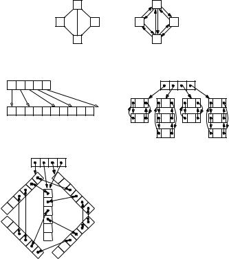
Fig. 8.1. The first row shows an undirected graph and the corresponding bidirected graph. The second row shows the adjacency array and adjacency list representations of this bidirected graph. The third row shows the linked-edge-objects representation and the adjacency matrix
edge array E. An additional array V stores the starting positions of the subarrays, i.e., for any node v, V [v] is the index in E of the first edge out of V . It is convenient to add a dummy entry V [n + 1] with V [n + 1] = m + 1. The edges out of any node v are then easily accessible as E[V [v]], . . . , E[V [v + 1] − 1]; the dummy entry ensures that this also holds true for node n. Figure 8.1 shows an example.
The memory consumption for storing a directed graph using adjacency arrays is n + m + Θ(1) words. This is even more compact than the 2m words needed for an edge sequence representation.
Adjacency array representations can be generalized to store additional information: we may store information associated with edges in separate arrays or within the edge array. If we also need incoming edges, we may use additional arrays V and E to store the reversed graph.
Exercise 8.1. Design a linear-time algorithm for converting an edge sequence representation of a directed graph into an adjacency array representation. You should use
170 8 Graph Representation
only O(1) auxiliary space. Hint: view the problem as the task of sorting edges by their source node and adapt the integer-sorting algorithm shown in Fig. 5.15.
8.3 Adjacency Lists – Dynamic Graphs
Edge arrays are a compact and efficient graph representation. Their main disadvantage is that it is expensive to add or remove edges. For example, assume that we want to insert a new edge (u, v). Even if there is room in the edge array E to accommodate it, we still have to move the edges associated with nodes u + 1 to n one position to the right, which takes time O(m).
In Chap. 3, we learned how to implement dynamic sequences. We can use any of the solutions presented there to produce a dynamic graph data structure. For each node v, we represent the sequence Ev of outgoing (or incoming, or outgoing and incoming) edges by an unbounded array or by a (singly or doubly) linked list. We inherit the advantages and disadvantages of the respective sequence representations. Unbounded arrays are more cache-efficient. Linked lists allow constant-time insertion and deletion of edges at arbitrary positions. Most graphs arising in practice are sparse in the sense that every node has only a few incident edges. Adjacency lists for sparse graphs should be implemented without the dummy item introduced in Sect. 3.1, because an additional item would waste considerable space. In the example in Fig. 8.1, we show circularly linked lists.
Exercise 8.2. Suppose the edges adjacent to a node u are stored in an unbounded array Eu, and an edge e = (u, v) is specified by giving its position in Eu. Explain how to remove e = (u, v) in constant amortized time. Hint: you do not have to maintain the relative order of the other edges.
Exercise 8.3. Explain how to implement the algorithm for testing whether a graph is acyclic discussed in Chap. 2.9 so that it runs in linear time, i.e., design an appropriate graph representation and an algorithm using it efficiently. Hint: maintain a queue of nodes with outdegree zero.
Bidirected graphs arise frequently. Undirected graphs are naturally presented as bidirected graphs, and some algorithms that operate on directed graphs need access not only to outgoing edges but also to incoming edges. In these situations, we frequently want to store the information associated with an undirected edge or a directed edge and its reversal only once. Also, we may want to have easy access from an edge to its reversal.
We shall describe two solutions. The first solution simply associates two additional pointers with every directed edge. One points to the reversal, and the other points to the information associated with the edge.
The second solution has only one item for each undirected edge (or pair of directed edges) and makes this item a member of two adjacency lists. So, the item for an undirected edge {u, v} would be a member of lists Eu and Ev. If we want doubly
8.4 The Adjacency Matrix Representation |
171 |
linked adjacency information, the edge object for any edge {u, v} stores four pointers: two are used for the doubly linked list representing Eu, and two are used for the doubly linked list representing Ev. Any node stores a pointer to some edge incident on it. Starting from it, all edges incident on the node can be traversed. The bottom part of Fig. 8.1 gives an example. A small complication lies in the fact that finding the other end of an edge now requires some work. Note that the edge object for an edge {u, v} stores the endpoints in no particular order. Hence, when we explore the edges out of a node u, we must inspect both endpoints and then choose the one which is different from u. An elegant alternative is to store u v in the edge object [145]. An exclusive OR with either endpoint then yields the other endpoint. Also, this representation saves space.
8.4 The Adjacency Matrix Representation
An n-node graph can be represented by an n×n adjacency matrix A. Ai j is 1 if (i, j) E and 0 otherwise. Edge insertion or removal and edge queries work in constant time. It takes time O(n) to obtain the edges entering or leaving a node. This is only efficient for very dense graphs with m = Ω n2 . The storage requirement is n2 bits. For very dense graphs, this may be better than the n + m + O(1) words required for adjacency arrays. However, even for dense graphs, the advantage is small if additional edge information is needed.
Exercise 8.4. Explain how to represent an undirected graph with n nodes and without self-loops using n(n − 1)/2 bits.
Perhaps more important than actually storing the adjacency matrix is the conceptual link between graphs and linear algebra introduced by the adjacency matrix. On the one hand, graph-theoretic problems can be solved using methods from linear algebra. For example, if C = Ak, then Ci j counts the number of paths from i to j with exactly k edges.
Exercise 8.5. Explain how to store an n × n matrix A with m nonzero entries using storage O(m + n) such that a matrix–vector multiplication Ax can be performed in time O(m + n). Describe the multiplication algorithm. Expand your representation so that products of the form xT A can also be computed in time O(m + n).
On the other hand, graph-theoretic concepts can be useful for solving problems from linear algebra. For example, suppose we want to solve the matrix equation Bx = c, where B is a symmetric matrix. Now consider the corresponding adjacency matrix A where Ai j = 1 if and only if Bi j =0. If an algorithm for computing connected components finds that the undirected graph represented by A contains two distinct connected components, this information can be used to reorder the rows and columns of B such that we obtain an equivalent equation of the form
B1 |
0 |
x1 |
= |
c1 |
. |
|
0 |
B2 |
x2 |
c2 |
|||
|
|
172 8 Graph Representation
This equation can now be solved by solving B1x1 = c1 and B2x2 = c2 separately. In practice, the situation is more complicated, since we rarely have matrices whose corresponding graphs are disconnected. Still, more sophisticated graph-theoretic concepts such as cuts can help to discover structure in the matrix which can then be exploited in solving problems in linear algebra.
8.5 Implicit Representations
Many applications work with graphs of special structure. Frequently, this structure can be exploited to obtain simpler and more efficient representations. We shall give two examples.
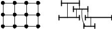
The grid graph Gk with node set V = [0..k − 1] × [0.. − 1] and edge set
E = ((i, j), (i, j )) V 2 : | j − j | = 1 ((i, j), (i , j)) V 2 : |i − i | = 1
is completely defined by the two parameters k and . Figure 8.2 shows G3,4. Edge weights could be stored in two two-dimensional arrays, one for the vertical edges and one for the horizontal edges.
An interval graph is defined by a set of intervals. For each interval, we have a node in the graph, and two nodes are adjacent if the corresponding intervals overlap.
Fig. 8.2. The grid graph G34 (left) and an interval graph with five nodes and six edges (right)
Exercise 8.6 (representation of interval graphs).
(a)Show that for any set of n intervals there is a set of intervals whose endpoints are integers in [1..2n] and that defines the same graph.
(b)Devise an algorithm that decides whether the graph defined by a set of n intervals is connected. Hint: sort the endpoints of the intervals and then scan over the endpoints in sorted order. Keep track of the number of intervals that have started
but not ended.
(c*) Devise a representation for interval graphs that needs O(n) space and supports efficient navigation. Given an interval I, you need to find all intervals I intersecting it; I intersects I if I contains an endpoint of I or I I . How can you find the former and the latter kinds of interval?
8.6 Implementation Notes
We have seen several representations of graphs in this chapter. They are suitable for different sets of operations on graphs, and can be tuned further for maximum