

Algorithms and data structures
.pdf214 10 Shortest Paths
A reÞned implementation of the BellmanÐFord algorithm [187, 131] explicitly maintains a current approximation T of the shortest-path tree. Nodes still to be scanned in the current iteration of the main loop are stored in a set Q. Consider the relaxation of an edge e = (u, v) that reduces d[v]. All descendants of v in T will subsequently receive a new d-value. Hence, there is no reason to scan these nodes with their current d-values and one may remove them from Q and T . Furthermore, negative cycles can be detected by checking whether v is an ancestor of u in T .
10.9.1 C++
LEDA [118] has a special priority queue class node_pq that implements priority queues of graph nodes. Both LEDA and the Boost graph library [27] have implementations of the Dijkstra and BellmanÐFord algorithms and of the algorithms for acyclic graphs and the all-pairs problem. There is a graph iterator based on DijkstraÕs algorithm that allows more ßexible control of the search process. For example, one can use it to search until a given set of target nodes has been found. LEDA also provides a function that veriÞes the correctness of distance functions (see Exercise 10.8).
10.9.2 Java
JDSL [78] provides DijkstraÕs algorithm for integer edge costs. This implementation allows detailed control over the search similarly to the graph iterators of LEDA and Boost.
10.10 Historical Notes and Further Findings
Dijkstra [56], Bellman [18], and Ford [63] found their algorithms in the 1950s. The original version of DijkstraÕs algorithm had a running time O m + n2 and there is a long history of improvements. Most of these improvements result from better data structures for priority queues. We have discussed binary heaps [208], Fibonacci heaps [68], bucket heaps [52], and radix heaps [9]. Experimental comparisons can be found in [40, 131]. For integer keys, radix heaps are not the end of the story. The best theoretical result is O(m + n log log n) time [194]. Interestingly, for undirected graphs, linear time can be achieved [190]. The latter algorithm still scans nodes one after the other, but not in the same order as in DijkstraÕs algorithm.
Meyer [139] gave the Þrst shortest-path algorithm with linear average-case running time. The algorithm ALD was found by Goldberg [76]. For graphs with bounded degree, the -stepping algorithm [140] is even simpler. This uses bucket queues and also yields a good parallel algorithm for graphs with bounded degree and small diameter.
Integrality of edge costs is also of use when negative edge costs are allowed.
If all edge costs are integers greater than −N, a scaling algorithm achieves a time
√
O(m n log N) [75].
10.10 Historical Notes and Further Findings |
215 |
In Sect. 10.8, we outlined a small number of speedup techniques for route planning. Many other techniques exist. In particular, we have not done justice to advanced goal-directed techniques, combinations of different techniques, etc. Recent overviews can be found in [166, 173]. Theoretical performance guarantees beyond DijkstraÕs algorithm are more difÞcult to achieve. Positive results exist for special families of graphs such as planar graphs and when approximate shortest paths sufÞce [60, 195, 192].
There is a generalization of the shortest-path problem that considers several cost functions at once. For example, your grandfather might want to know the fastest route for visiting you but he only wants routes where he does not need to refuel his car, or you may want to know the fastest route subject to the condition that the road toll does not exceed a certain limit. Constrained shortest-path problems are discussed in [86, 135].
Shortest paths can also be computed in geometric settings. In particular, there is an interesting connection to optics. Different materials have different refractive indices, which are related to the speed of light in the material. Astonishingly, the laws of optics dictate that a ray of light always travels along a shortest path.
Exercise 10.21. An ordered semigroup is a set S together with an associative and commutative operation +, a neutral element 0, and a linear ordering ≤ such that for all x, y, and z, x ≤ y implies x + z ≤ y + z. Which of the algorithms of this chapter work when the edge weights are from an ordered semigroup? Which of them work under the additional assumption that 0 ≤ x for all x?
11
Minimum Spanning Trees
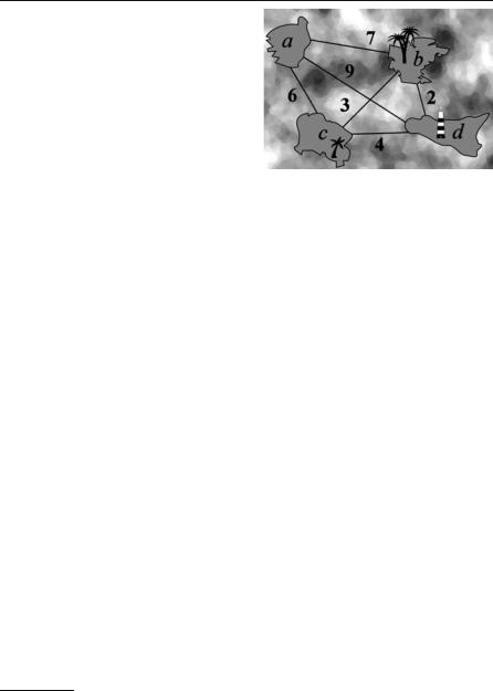
The atoll of Taka-Tuka-Land in the South Seas asks you for help.1 The people want to connect their islands by ferry lines. Since money is scarce, the total cost of the connections is to be minimized. It needs to be possible to travel between any two islands; direct connections are not necessary. You are given a list of possible connections together with their estimated costs. Which connections should be opened?
More generally, we want to solve the following problem. Consider a connected undirected graph G = (V, E) with real edge costs c : E → R+. A minimum spanning tree (MST) of G is defined by a set T E of edges such that the graph (V, T ) is a tree where c(T ) := ∑e T c(e) is minimized. In our example, the nodes are islands, the edges are possible ferry connections, and the costs are the costs of opening a connection. Throughout this chapter, G denotes an undirected connected graph.
Minimum spanning trees are perhaps the simplest variant of an important family of problems known as network design problems. Because MSTs are such a simple concept, they also show up in many seemingly unrelated problems such as clustering, finding paths that minimize the maximum edge cost used, and finding approximations for harder problems. Sections 11.6 and 11.8 discuss this further. An equally good reason to discuss MSTs in a textbook on algorithms is that there are simple, elegant, fast algorithms to find them. We shall derive two simple properties of MSTs in Sect. 11.1. These properties form the basis of most MST algorithms. The Jarník–Prim algorithm grows an MST starting from a single node and will be discussed in Sect. 11.2. Kruskal’s algorithm grows many trees in unrelated parts of the graph at once and merges them into larger and larger trees. This will be discussed in Sect. 11.3. An efficient implementation of the algorithm requires a data structure for maintaining partitions of a set of elements under two operations: “determine whether two elements are in the same subset” and “join two subsets”. We shall discuss the union–find data structure in Sect. 11.4. This has many applications besides the construction of minimum spanning trees.
1 The figure was drawn by A. Blancani.
218 11 Minimum Spanning Trees
Exercise 11.1. If the input graph is not connected, we may ask for a minimum spanning forest – a set of edges that defines an MST for each connected component of G. Develop a way to find minimum spanning forests using a single call of an MST routine. Do not find connected components first. Hint: insert n − 1 additional edges.
Exercise 11.2 (spanning sets). A set T of edges spans a connected graph G if (V, T ) is connected. Is a minimum-cost spanning set of edges necessarily a tree? Is it a tree if all edge costs are positive?
Exercise 11.3. Reduce the problem of finding maximum-cost spanning trees to the minimum-spanning-tree problem.
11.1 Cut and Cycle Properties
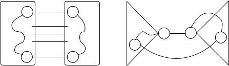
We shall prove two simple Lemmas which allow one to add edges to an MST and to exclude edges from consideration for an MST. We need the concept of a cut in a graph. A cut in a connected graph is a subset E of edges such that G \ E is not connected. Here, G \ E is an abbreviation for (V, E \ E ). If S is a set of nodes with 0/ = S = V , the set of edges with exactly one endpoint in S forms a cut. Figure 11.1 illustrates the proofs of the following lemmas.
Lemma 11.1 (cut property). Let E be a cut and let e be a minimal-cost edge in E . There is then an MST T of G that contains e. Moreover, if T is a set of edges that is contained in some MST and T contains no edge from E , then T {e} is also contained in some MST.
Proof. We shall prove the second claim. The first claim follows by setting T = 0/. Consider any MST T of G with T T . Let u and v be the endpoints of e. Since T is a spanning tree, it contains a path from u to v, say p. Since E is a cut separating u and
|
E |
|
|
|
|
u |
e |
v |
|
|
C |
|
|
|
|
||
p |
|
p |
u |
e |
v |
|
|
||||
u |
e |
v |
|
e |
|
|
|
Tv |
|||
|
Tu |
|
|
||
|
|
|
|
Fig. 11.1. Cut and cycle properties. The left part illustrates the proof of the cut property. e is an edge of minimum cost in the cut E , and p is a path in the MST connecting the endpoints of e. p must contain an edge in E . The figure on the right illustrates the proof of the cycle property. C is a cycle in G, e is an edge of C of maximal weight, and T is an MST containing e. Tu and Tv are the components of T \ e; and e is an edge in C connecting Tu and Tv

11.2 The Jarník–Prim Algorithm |
219 |
v, p must contain an edge from E , say e . Now, T := (T \ e ) e is also a spanning
tree, because removal of e splits T into two subtrees, which are then joined together by e. Since c(e) ≤ c(e ), we have c(T ) ≤ c(T ), and hence T is also an MST.
Lemma 11.2 (cycle property). Consider any cycle C E and an edge e C with maximal cost among all edges of C. Then any MST of G = (V, E \ {e}) is also an MST of G.
Proof. Consider any MST T of G. Suppose T contains e = (u, v). Edge e splits T into two subtrees Tu and Tv. There must be another edge e = (u , v ) from C such that
u Tu and v Tv. T := (T \ {e}) {e } is a spanning tree which does not contain e. Since c(e ) ≤ c(e), T is also an MST.
The cut property yields a simple greedy algorithm for finding an MST. Start with an empty set T of edges. As long as T is not a spanning tree, let E be a cut not containing any edge from T . Add a minimal-cost edge from E to T .
Different choices of E lead to different specific algorithms. We discuss two approaches in detail in the following sections and outline a third approach in Sect. 11.8. Also, we need to explain how to find a minimum cost edge in the cut.
The cycle property also leads to a simple algorithm for finding an MST. Set T to the set of all edges. As long as T is not a spanning tree, find a cycle in T and delete an edge of maximal cost from T . No efficient implementation of this approach is known, and we shall not discuss it further.
Exercise 11.4. Show that the MST is uniquely defined if all edge costs are different. Show that in this case the MST does not change if each edge cost is replaced by its rank among all edge costs.
11.2 The Jarník–Prim Algorithm
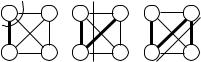
The Jarník–Prim (JP) algorithm [98, 158, 56] for MSTs is very similar to Dijkstra’s algorithm for shortest paths.2 Starting from an (arbitrary) source node s, the JP algorithm grows an MST by adding one node after another. At any iteration, S is the set of nodes already added to the tree, and the cut E is the set of edges with exactly one endpoint in S. A minimum-cost edge leaving S is added to the tree in every iteration. The main challenge is to find this edge efficiently. To this end, the algorithm maintains the shortest connection between any node v V \ S and S in a priority queue Q. The smallest element in Q gives the desired edge. When a node is added to S, its incident edges are checked to see whether they yield improved connections to nodes in V \S. Fig. 11.2 illustrates the operation of the JP algorithm, and Figure 11.3 shows the pseudocode. When node u is added to S and an incident edge e = (u, v) is inspected, the algorithm needs to know whether v S. A bitvector could be used to
2Actually, Dijkstra also described this algorithm in his seminal 1959 paper on shortest paths [56]. Since Prim described the same algorithm two years earlier, it is usually named after him. However, the algorithm actually goes back to a 1930 paper by Jarník [98].
220 11 Minimum Spanning Trees
encode this information. If all edge costs are positive, we can reuse the d-array for this purpose. For any node v, d[v] = 0 indicates v S and d[v] > 0 encodes v S.
In addition to the space savings, this trick also avoids a comparison in the innermost loop. Observe that c(e) < d[v] is only true if d[v] > 0, i.e., v S, and e is an improved connection from v to S.
The only important difference from Dijkstra’s algorithm is that the priority queue stores edge costs rather than path lengths. The analysis of Dijkstra’s algorithm carries over to the JP algorithm, i.e., the use of a Fibonacci heap priority queue yields a running time O(n log n + m).
Exercise 11.5. Dijkstra’s algorithm for shortest paths can use monotone priority queues. Show that monotone priority queues do not suffice for the JP algorithm.
*Exercise 11.6 (average-case analysis of the JP algorithm). Assume that the edge costs 1, . . . , m are assigned randomly to the edges of G. Show that the expected number of decreaseKey operations performed by the JP algorithm is then bounded by O(n log(m/n)). Hint: the analysis is very similar to the average-case analysis of Dijkstra’s algorithm in Theorem 10.6.
a |
7 |
b |
a |
7 |
b |
|
a |
7 |
b |
6 |
9 |
2 |
6 |
9 |
2 |
6 |
|
9 |
2 |
3 |
3 |
|
3 |
||||||
c |
d |
c |
d |
|
c |
d |
|||
|
4 |
|
|
4 |
|
|
|
4 |
|
Fig. 11.2. A sequence of cuts (dotted lines) corresponding to the steps carried out by the Jarník–Prim algorithm with starting node a. The edges (a, c), (c, b), and (b, d) are added to the MST
Function jpMST : Set of Edge |
|
|
d = ∞, . . . , ∞ : NodeArray[1..n] of R {∞} |
// d[v] is the distance of v from the tree |
|
parent : NodeArray of NodeId |
// |
parent[v] is shortest edge between S and v |
Q : NodePQ |
|
// uses d[·] as priority |
Q.insert(s) for some arbitrary s V |
|
|
while Q = 0/ do |
|
|
u := Q.deleteMin |
|
// d[u] = 0 encodes u S |
d[u] := 0 |
|
|
foreach edge e = (u, v) E do |
// c(e) < d[v] implies d[v] > 0 and hence v S |
|
if c(e) < d[v] then |
||
d[v] := c(e) |
|
|
parent[v] := u |
|
|
if v Q then Q.decreaseKey(v) else Q.insert(v) invariant v Q : d[v] = min {c((u, v)) : (u, v) E u S}
return {(v, parent[v]) : v V \ {s}}
Fig. 11.3. The Jarník–Prim MST algorithm. Positive edge costs are assumed
11.3 Kruskal’s Algorithm |
221 |
11.3 Kruskal’s Algorithm
The JP algorithm is probably the best general-purpose MST algorithm. Nevertheless, we shall now present an alternative algorithm, Kruskal’s algorithm [116]. It also has its merits. In particular, it does not need a sophisticated graph representation, but works even when the graph is represented by its sequence of edges. Also, for sparse graphs with m = O(n), its running time is competitive with the JP algorithm.
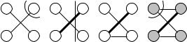
The pseudocode given in Fig. 11.4 is extremely compact. The algorithm scans over the edges of G in order of increasing cost and maintains a partial MST T ; T is initially empty. The algorithm maintains the invariant that T can be extended to an MST. When an edge e is considered, it is either discarded or added to the MST. The decision is made on the basis of the cycle or cut property. The endpoints of e either belong to the same connected component of (V, T ) or do not. In the former case, T e contains a cycle and e is an edge of maximum cost in this cycle. Since edges are considered in order of increasing cost, e can be discarded, by the cycle property. If e connects distinct components, e is a minimum-cost edge in the cut E consisting of all edges connecting distinct components of (V, T ); again, it is essential that edges are considered in order of increasing cost. We may therefore add e to T , by the cut property. The invariant is maintained. Figure 11.5 gives an example.
In an implementation of Kruskal’s algorithm, we have to find out whether an edge connects two components of (V, T ). In the next section, we shall see that this can be done so efficiently that the main cost factor is sorting the edges. This takes time O(m log m) if we use an efficient comparison-based sorting algorithm. The constant factor involved is rather small, so that for m = O(n) we can hope to do better than the O(m + n log n) JP algorithm.
Function kruskalMST(V, E, c) : Set of Edge |
|
|
|
|
|
|
|
|
|
|
|
||||||||||
T := 0/ |
|
|
|
|
|
|
|
|
|
|
|
|
|
|
|
|
|
|
|
||
invariant T is a subforest of an MST |
|
|
|
|
|
|
|
|
|
|
|
|
|
||||||||
foreach (u, v) E in ascending order of cost do |
|
|
|
|
|
|
|
|
|||||||||||||
if u and v are in different subtrees of T then |
|
|
|
|
|
|
|
|
|||||||||||||
T := T {(u, v)} |
|
|
|
|
|
|
|
|
|
|
|
|
|
|
|
// join two subtrees |
|||||
return T |
|
|
|
|
|
|
|
|
|
|
|
|
|
|
|
|
|
|
|
||
|
|
|
|
Fig. 11.4. Kruskal’s MST algorithm |
|
|
|
||||||||||||||
a |
7 |
b |
a |
7 |
b |
a |
|
7 |
b |
a |
7 |
b |
|||||||||
9 |
9 |
|
9 |
9 |
|||||||||||||||||
6 |
|
|
2 |
6 |
|
|
2 |
6 |
|
|
|
2 |
6 |
|
|
2 |
|||||
|
3 |
|
|
3 |
|
|
|
3 |
|
|
3 |
|
|||||||||
|
|
|
|
|
|
|
|
|
|
|
|
|
|
|
|
||||||
c |
d |
c |
d |
c |
d |
c |
d |
||||||||||||||
4 |
4 |
4 |
4 |
||||||||||||||||||
|
|
|
|
|
|
|
|
|
|||||||||||||
Fig. 11.5. In this example, Kruskal’s algorithm first proves that (b, d) and (b, c) are MST edges using the cut property. Then (c, d) is excluded because it is the heaviest edge on the cycle b, c, d , and, finally, (a, c) completes the MST

222 11 Minimum Spanning Trees
Exercise 11.7 (streaming MST). Suppose the edges of a graph are presented to you only once (for example over a network connection) and you do not have enough memory to store all of them. The edges do not necessarily arrive in sorted order.
(a) Outline an algorithm that nevertheless computes an MST using space O(V ). (*b) Refine your algorithm to run in time O(m log n). Hint: process batches of O(n)
edges (or use the dynamic tree data structure described by Sleator and Tarjan [182]).
11.4 The Union–Find Data Structure
A partition of a set M is a collection M1, . . . , Mk of subsets of M with the property that the subsets are disjoint and cover M, i.e., Mi ∩Mj = 0/ for i = j and M = M1 ···Mk. The subsets Mi are called the blocks of the partition. For example, in Kruskal’s algorithm, the forest T partitions V . The blocks of the partition are the connected components of (V, T ). Some components may be trivial and consist of a single isolated node. Kruskal’s algorithm performs two operations on the partition: testing whether two elements are in the same subset (subtree) and joining two subsets into one (inserting an edge into T ).
The union–find data structure maintains a partition of the set 1..n and supports these two operations. Initially, each element is a block on its own. Each block chooses one of its elements as its representative; the choice is made by the data structure and not by the user. The function find(i) returns the representative of the block containing i. Thus, testing whether two elements are in the same block amounts to comparing their respective representatives. An operation link(i, j) applied to representatives of different blocks joins the blocks.
A simple solution is as follows. Each block is represented as a rooted tree3, with the root being the representative of the block. Each element stores its parent in this tree (the array parent). We have self-loops at the roots.
The implementation of find(i) is trivial. We follow parent pointers until we encounter a self-loop. The self-loop is located at the representative of i. The implementation of link(i, j) is equally simple. We simply make one representative the parent of the other. The latter has ceded its role to the former, which is now the representative of the combined block. What we have described so far yields a correct but inefficient union–find data structure. The parent references could form long chains that are traversed again and again during find operations. In the worst case, each operation may take linear time.
Exercise 11.8. Give an example of an n-node graph with O(n) edges where a naive implementation of the union–find data structure without union by rank and path compression would lead to quadratic execution time for Kruskal’s algorithm.
3Note that this tree may have a structure very different from the corresponding subtree in Kruskal’s algorithm.

|
|
11.4 |
The Union–Find Data Structure |
223 |
||||
Class UnionFind(n : N) |
|
// Maintain a partition of 1..n |
|
|
||||
parent = 1, 2, . . . , n : Array [1..n] of 1..n |
|
rank of representatives 1 2 |
... |
|
||||
|
n |
|||||||
rank = 0, . . . , 0 : Array [1..n] of 0.. log n |
// |
|||||||
Function find(i : 1..n) : 1..n |
|
|
|
|
i |
|
|
|
if parent[i] = i then return i |
|
|
|
|
... |
|
||
|
|
|
. |
|
||||
else i := find(parent[i]) |
// path compression |
|
||||||
|
|
|||||||
parent[i] := i |
|
|
|
|
parent[i] |
|
|
|
return i |
|
|
|
|
|
|
||
|
|
|
|
i |
|
|
||
|
|
|
|
|
|
|
||
Procedure link(i, j : 1..n) |
|
|
|
|
assert i and j are representatives of different blocks |
i |
2 |
|
j |
if rank[i] < rank[ j] then parent[i] := j |
3 |
|||
else |
|
|
|
|
parent[ j] := i |
|
|
|
|
if rank[i] = rank[ j] then rank[i]++ |
i |
2 |
2 |
j |
|
i |
j |
|
3 |
i |
3 |
j |
Procedure union(i, j : 1..n)
if find(i) = find( j) then link(find(i), find( j))
Fig. 11.6. An efficient union–find data structure that maintains a partition of the set {1, . . . , n}
Therefore, Figure 11.6 introduces two optimizations. The first optimization limits the maximal depth of the trees representing blocks. Every representative stores a nonnegative integer, which we call its rank. Initially, every element is a representative and has rank zero. When we link two representatives and their ranks are different, we make the representative of smaller rank a child of the representative of larger rank. When their ranks are the same, the choice of the parent is arbitrary; however, we increase the rank of the new root. We refer to the first optimization as union by rank.
Exercise 11.9. Assume that the second optimization (described below) is not used. Show that the rank of a representative is the height of the tree rooted at it.
Theorem 11.3. Union by rank ensures that the depth of no tree exceeds log n.
Proof. Without path compression, the rank of a representative is equal to the height of the tree rooted at it. Path compression does not increase heights. It therefore suffices to prove that the rank is bounded by log n. We shall show that a tree whose root has rank k contains at least 2k elements. This is certainly true for k = 0. The rank of a root grows from k − 1 to k when it receives a child of rank k − 1. Thus the root had at least 2k−1 descendants before the link operation and it receives a child which also had at least 2k−1 descendants. So the root has at least 2k descendants after the link operation.
The second optimization is called path compression. This ensures that a chain of parent references is never traversed twice. Rather, all nodes visited during an op-

224 11 Minimum Spanning Trees
eration find(i) redirect their parent pointers directly to the representative of i. In Fig. 11.6, we have formulated this rule as a recursive procedure. This procedure first traverses the path from i to its representative and then uses the recursion stack to traverse the path back to i. When the recursion stack is unwound, the parent pointers are redirected. Alternatively, one can traverse the path twice in the forward direction. In the first traversal, one finds the representative, and in the second traversal, one redirects the parent pointers.
Exercise 11.10. Describe a nonrecursive implementation of find.
Union by rank and path compression make the union–find data structure “breathtakingly” efficient – the amortized cost of any operation is almost constant.
Theorem 11.4. The union–find data structure of Fig. 11.6 performs m find and n −1 link operations in time O(mαT (m, n)). Here,
αT (m, n) = min {i ≥ 1 : A(i, m/n ) ≥ log n},
where
A(1, j) = 2 j |
for j ≥ 1, |
A(i, 1) = A(i − 1, 2) |
for i ≥ 2, |
A(i, j) = A(i − 1, A(i, j − 1)) |
for i ≥ 2 and j ≥ 2. |
Proof. The proof of this theorem is beyond the scope of this introductory text. We refer the reader to [186, 177].
You will probably find the formulae overwhelming. The function4 A grows extremely rapidly. We have A(1, j) = 2 j, A(2, 1) = A(1, 2) = 22 = 4, A(2, 2) = A(1, A(2, 1)) = 24 = 16, A(2, 3) = A(1, A(2, 2)) = 216, A(2, 4) = 2216 , A(2, 5) = 22216 ,
A(3, 1) = A(2, 2) = 16, A(3, 2) = A(2, A(3, 1)) = A(2, 16), and so on.
Exercise 11.11. Estimate A(5, 1).
For all practical n, we have αT (m, n) ≤ 5, and union–find with union by rank and path compression essentially guarantees constant amortized cost per operation.
We close this section with an analysis of union–find with path compression but without union by rank. The analysis illustrates the power of path compression and also gives a glimpse of how Theorem 11.4 can be proved.
Theorem 11.5. The union–find data structure with path compression but without union by rank processes m find and n − 1 link operations in time O((m + n) log n).
4The usage of the letter A is a reference to the logician Ackermann [3], who first studied a variant of this function in the late 1920s.