Algorithms and data structures

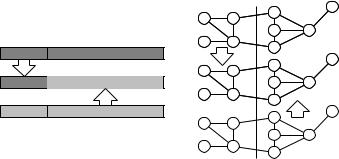
Fig. 12.11. The Þgure on the left shows a partial coloring of the graph underlying sudoku puzzles. The bold straight-line segments indicate cliques consisting of all nodes touched by the line. The Þgure on the right shows a step of Kempe chain annealing using colors 1 and 2 and a node v

accepted. Furthermore, one can use a simpliÞed statistical model of the process to estimate when the system is approaching equilibrium. The details of dynamic schedules are beyond the scope of this exposition. Readers are referred to [1] for more details on simulated annealing.

Exercise 12.23. Design a simulated-annealing algorithm for the knapsack problem. The local neighborhood of a feasible solution is all solutions that can be obtained by removing up to two elements and then adding up to two elements.

Graph Coloring

We shall now exemplify simulated annealing on the graph-coloring problem already mentioned in Sect. 2.10. Recall that we are given an undirected graph G = (V, E) and are looking for an assignment c : V → 1..k such that no two adjacent nodes are given the same color, i.e., c(u) =c(v) for all edges {u, v} E. There is always a solution with k = |V | colors; we simply give each node its own color. The goal is to minimize k. There are many applications of graph coloring and related problems. The most ÒclassicalÓ one is map coloring Ð the nodes are countries and edges indicate that these countries have a common border, and thus these countries should not be rendered in the same color. A famous theorem of graph theory states that all maps (i.e. planar graphs) can be colored with at most four colors [162]. Sudoku puzzles are a well-known instance of the graph-coloring problem, where the player is asked to complete a partial coloring of the graph shown in Fig. 12.11 with the digits 1..9. We shall present two simulated-annealing approaches to graph coloring; many more have been tried.

Kempe Chain Annealing

Of course, the obvious objective function for graph coloring is the number of colors used. However, this choice of objective function is too simplistic in a local-search

256 12 Generic Approaches to Optimization

framework, since a typical local move will not change the number of colors used. We need an objective function that rewards local changes that are Òon a good wayÓ towards using fewer colors. One such function is the sum of the squared sizes of the color classes. Formally, let Ci = {v V : c(v) = i} be the set of nodes that are

colored i. Then

f (c) = ∑|Ci|2 .

i

This objective function is to be maximized. Observe that the objective function increases when a large color class is enlarged further at the cost of a small color class. Thus local improvements will eventually empty some color classes, i.e., the number of colors decreases.

Having settled the objective function, we come to the deÞnition of a local change or a neighborhood. A trivial deÞnition is as follows: a local change consists in recoloring a single vertex; it can be given any color not used on one of its neighbors. Kempe chain annealing uses a more liberal deÞnition of Òlocal recoloringÓ. Alfred Bray Kempe (1849Ð1922) was one of the early investigators of the four-color problem; he invented Kempe chains in his futile attempts at a proof. Suppose that we want to change the color c(v) of node v from i to j. In order to maintain feasibility, we have to change some other node colors too: node v might be connected to nodes currently colored j. So we color these nodes with color i. These nodes might, in turn, be connected to other nodes of color j, and so on. More formally, consider the node-induced subgraph H of G which contains all nodes with colors i and j. The connected component of H that contains v is the Kempe chain K we are interested in. We maintain feasibility by swapping colors i and j in K. Figure 12.11 gives an example. Kempe chain annealing starts with any feasible coloring.

*Exercise 12.24. Use Kempe chains to prove that any planar graph G can be colored with Þve colors. Hint: use the fact that a planar graph is guaranteed to have a node of degree Þve or less. Let v be any such node. Remove it from G, and color G − v recursively. Put v back in. If at most four different colors are used on the neighbors of v, there is a free color for v. So assume otherwise. Assume, without loss of generality, that the neighbors of v are colored with colors 1 to 5 in clockwise order. Consider the subgraph of nodes colored 1 and 3. If the neighbors of v with colors 1 and 3 are in distinct connected components of this subgraph, a Kempe chain can be used to recolor the node colored 1 with color 3. If they are in the same component, consider the subgraph of nodes colored 2 and 4. Argue that the neighbors of v with colors 2 and 4 must be in distinct components of this subgraph.

The Penalty Function Approach

A generally useful idea for local search is to relax some of the constraints on feasible solutions in order to make the search more ßexible and to ease the discovery of a starting solution. Observe that we have assumed so far that we somehow have a feasible solution available to us. However, in some situations, Þnding any feasible solution is already a hard problem; the eight-queens problem of Exercise 12.21 is an example. In order to obtain a feasible solution at the end of the process, the objective

function is modiÞed to penalize infeasible solutions. The constraints are effectively moved into the objective function.

In the graph-coloring example, we now also allow illegal colorings, i.e., colorings in which neighboring nodes may have the same color. An initial solution is generated by guessing the number of colors needed and coloring the nodes randomly. A neighbor of the current coloring c is generated by picking a random color j and a random node v colored j, i.e., x(v) = j. Then, a random new color for node v is chosen from all the colors already in use plus one fresh, previously unused color.

As above, let Ci be the set of nodes colored i and let Ei = E ∩Ci ×Ci be the set of edges connecting two nodes in Ci. The objective is to minimize

f (c) = 2 ∑|Ci| · |Ei| − ∑|Ci|2 .

The Þrst term penalizes illegal edges; each illegal edge connecting two nodes of color i contributes the size of the i-th color class. The second term favors large color classes, as we have already seen above. The objective function does not necessarily have its global minimum at an optimal coloring, however, local minima are legal colorings. Hence, the penalty version of simulated annealing is guaranteed to Þnd a legal coloring even if it starts with an illegal coloring.

Exercise 12.25. Show that the objective function above has its local minima at legal colorings. Hint: consider the change in f (c) if one end of a legally colored edge is recolored with a fresh color. Prove that the objective function above does not necessarily have its global optimum at a solution using the minimal number of colors.

Experimental Results

Johnson et al. [101] performed a detailed study of algorithms for graph coloring, with particular emphasis on simulated annealing. We shall brießy report on their Þndings and then draw some conclusions. Most of their experiments were performed on random graphs in the Gn, p-model or on random geometric graphs.

In the Gn, p-model, where p is a parameter in [0, 1], an undirected random graph with n nodes is built by adding each of the n(n − 1)/2 candidate edges with probability p. The random choices for distinct edges are independent. In this way, the expected degree of every node is p(n − 1) and the expected number of edges is pn(n − 1)/2. For random graphs with 1 000 nodes and edge probability 0.5, Kempe chain annealing produced very good colorings, given enough time. However, a sophisticated and expensive greedy algorithm, XRLF, produced even better solutions in less time. For very dense random graphs with p = 0.9, Kempe chain annealing performed better than XRLF. For sparser random graphs with edge probability 0.1, penalty function annealing outperformed Kempe chain annealing and could sometimes compete with XRLF.

Another interesting class of random inputs is random geometric graphs. Here, we choose n random, uniformly distributed points in the unit square [0, 1] × [0, 1]. These points represent the nodes of the graph. We connect two points by an edge if their Euclidean distance is less than or equal to some given range r. Figure 12.12

gives an example. Such instances are frequently used to model situations where the nodes represent radio transmitters and colors represent frequency bands. Nodes that lie within a distance r from one another must not use the same frequency, to avoid interference. For this model, Kempe chain annealing performed well, but was outperformed by a third annealing strategy, called fixed-K annealing.

What should we learn from this? The relative performance of the simulatedannealing approaches depends strongly on the class of inputs and the available computing time. Moreover, it is impossible to make predictions about their performance on any given instance class on the basis of experience from other instance classes. So be warned. Simulated annealing is a heuristic and, as for any other heuristic, you should not make claims about its performance on an instance class before you have tested it extensively on that class.

12.5.3 More on Local Search

We close our treatment of local search with a discussion of three reÞnements that can be used to modify or replace the approaches presented so far.

Threshold Acceptance

There seems to be nothing magic about the particular form of the acceptance rule used in simulated annealing. For example, a simpler yet also successful rule uses the parameter T as a threshold. New states with a value f (x) below the threshold are accepted, whereas others are not.

Tabu Lists

Local-search algorithms sometimes return to the same suboptimal solution again and again Ð they cycle. For example, simulated annealing might have reached the top of a steep hill. Randomization will steer the search away from the optimum, but the state may remain on the hill for a long time. Tabu search steers the search away from local optima by keeping a tabu list of Òsolution elementsÓ that should be ÒavoidedÓ in new solutions for the time being. For example, in graph coloring, a search step could change the color of a node v from i to j and then store the tuple (v, i) in the tabu list to indicate that color i is forbidden for v as long as (v, i) is in the tabu list. Usually, this tabu condition is not applied if an improved solution is obtained by coloring node v

with color i. Tabu lists are so successful that they can be used as the core technique of an independent variant of local search called tabu search.

Restarts

The typical behavior of a well-tuned local-search algorithm is that it moves to an area with good feasible solutions and then explores this area, trying to Þnd better and better local optima. However, it might be that there are other, far away areas with much better solutions. The search for Mount Everest illustrates this point. If we start in Australia, the best we can hope for is to end up at Mount Kosciusko (altitude 2229 m), a solution far from optimum. It therefore makes sense to run the algorithm multiple times with different random starting solutions because it is likely that different starting points will explore different areas of good solutions. Starting the search for Mount Everest at multiple locations and in all continents will certainly lead to a better solution than just starting in Australia. Even if these restarts do not improve the average performance of the algorithm, they may make it more robust in the sense that it will be less likely to produce grossly suboptimal solutions. Several independent runs are also an easy source of parallelism: just run the program on several different workstations concurrently.

12.6 Evolutionary Algorithms

Living beings are ingeniously adaptive to their environment, and master the problems encountered in daily life with great ease. Can we somehow use the principles of life for developing good algorithms? The theory of evolution tells us that the mechanisms leading to this performance are mutation, recombination, and survival of the fittest. What could an evolutionary approach mean for optimization problems?

The genome describing an individual corresponds to the description of a feasible solution. We can also interpret infeasible solutions as dead or ill individuals. In nature, it is important that there is a sufÞciently large population of genomes; otherwise, recombination deteriorates to incest, and survival of the Þttest cannot demonstrate its beneÞts. So, instead of one solution as in local search, we now work with a pool of feasible solutions.

The individuals in a population produce offspring. Because resources are limited, individuals better adapted to the environment are more likely to survive and to produce more offspring. In analogy, feasible solutions are evaluated using a Þtness function f , and Þtter solutions are more likely to survive and to produce offspring. Evolutionary algorithms usually work with a solution pool of limited size, say N. Survival of the Þttest can then be implemented as keeping only the N best solutions.

Even in bacteria, which reproduce by cell division, no offspring is identical to its parent. The reason is mutation. When a genome is copied, small errors happen. Although mutations usually have an adverse effect on Þtness, some also improve Þtness. Local changes in a solution are the analogy of mutations.

260 12 Generic Approaches to Optimization

Create an initial population population = x1, . . . , xN while not Þnished do

if matingStep then

select individuals x1, x2 with high Þtness and produce x := mate(x1, x2) else select an individual x1 with high Þtness and produce x = mutate(x1) population := population {x }

population := {x population : x is sufÞciently Þt}

Fig. 12.13. A generic evolutionary algorithm

An even more important ingredient in evolution is recombination. Offspring contain genetic information from both parents. The importance of recombination is easy to understand if one considers how rare useful mutations are. Therefore it takes much longer to obtain an individual with two new useful mutations than it takes to combine two individuals with two different useful mutations.

We now have all the ingredients needed for a generic evolutionary algorithm; see Fig. 12.13. As with the other approaches presented in this chapter, many details need to be Þlled in before one can obtain an algorithm for a speciÞc problem. The algorithm starts by creating an initial population of size N. This process should involve randomness, but it is also useful to use heuristics that produce good initial solutions.

In the loop, it is Þrst decided whether an offspring should be produced by mutation or by recombination. This is a probabilistic decision. Then, one or two individuals are chosen for reproduction. To put selection pressure on the population, it is important to base reproductive success on the Þtness of the individuals. However, it is usually not desirable to draw a hard line and use only the Þttest individuals, because this might lead to too uniform a population and incest. For example, one can instead choose reproduction candidates randomly, giving a higher selection probability to Þtter individuals. An important design decision is how to Þx these probabilities. One choice is to sort the individuals by Þtness and then to deÞne the reproduction probability as some decreasing function of rank. This indirect approach has the advantage that it is independent of the objective function f and the absolute Þtness differences between individuals, which are likely to decrease during the course of evolution.

The most critical operation is mate, which produces new offspring from two ancestors. The ÒcanonicalÓ mating operation is called crossover. Here, individuals are assumed to be represented by a string of n bits. An integer k is chosen. The new individual takes its Þrst k bits from one parent and its last n − k bits from the other parent. Figure 12.14 shows this procedure. Alternatively, one may choose k random positions from the Þrst parent and the remaining bits from the other parent. For our knapsack example, crossover is a quite natural choice. Each bit decides whether the corresponding item is in the knapsack or not. In other cases, crossover is less natural or would require a very careful encoding. For example, for graph coloring, it would seem more natural to cut the graph into two pieces such that only a few edges are cut. Now one piece inherits its colors from the Þrst parent, and the other piece inherits its colors from the other parent. Some of the edges running between the pieces might

262 12 Generic Approaches to Optimization

•Develop a local-search algorithm. Focus on a good representation of solutions and how to incorporate application-speciÞc knowledge into the searcher. If you have a promising idea for a mating operator, you can also consider evolutionary algorithms. Use randomization and restarts to make the results more robust.

There are many implementations of linear-programming solvers. Since a good implementation is very complicated, you should deÞnitely use one of these packages except in very special circumstances. The Wikipedia page on Òlinear programmingÓ is a good starting point. Some systems for linear programming also support integer linear programming.

There are also many frameworks that simplify the implementation of local-search or evolutionary algorithms. Since these algorithms are fairly simple, the use of these frameworks is not as widespread as for linear programming. Nevertheless, the implementations available might have nontrivial built-in algorithms for dynamic setting of search parameters, and they might support parallel processing. The Wikipedia page on Òevolutionary algorithmÓ contains pointers.

12.8 Historical Notes and Further Findings

We have only scratched the surface of (integer) linear programming. Implementing solvers, clever modeling of problems, and handling huge input instances have led to thousands of scientiÞc papers. In the late 1940s, Dantzig invented the simplex algorithm [45]. Although this algorithm works well in practice, some of its variants take exponential time in the worst case. It is a famous open problem whether some variant runs in polynomial time in the worst case. It is known, though, that even slightly perturbing the coefÞcients of the constraints leads to polynomial expected execution time [184]. Sometimes, even problem instances with an exponential number of constraints or variables can be solved efÞciently. The trick is to handle explicitly only those constraints that may be violated and those variables that may be nonzero in an optimal solution. This works if we can efÞciently Þnd violated constraints or possibly nonzero variables and if the total number of constraints and variables generated remains small. Khachiyan [110] and Karmakar [106] found polynomial-time algorithms for linear programming. There are many good textbooks on linear programming (e.g. [23, 58, 73, 147, 172, 199]).

Another interesting blackbox solver is constraint programming [90, 121]. We hinted at the technique in Exercise 12.21. Here, we are again dealing with variables and constraints. However, now the variables come from discrete sets (usually small Þnite sets). Constraints come in a much wider variety. There are equalities and inequalities, possibly involving arithmetic expressions, but also higher-level constraints. For example, allDifferent(x1, . . . , xk) requires that x1, . . . , xk all receive different values. Constraint programs are solved using a cleverly pruned systematic search. Constraint programming is more ßexible than linear programming, but restricted to smaller problem instances. Wikipedia is a good starting point for learning more about constraint programming.

A

Appendix

A.1 Mathematical Symbols

{e0, . . . , en−1}: set containing elements e0, . . . , en−1.

{e : P(e)}: set of all elements that fulfill the predicate P.

e0, . . . , en−1 : sequence consisting of elements e0, . . . , en−1.

e S : P(e) : subsequence of all elements of sequence S that fulfill the predicate P.

|x|: the absolute value of x.

x : the largest integer ≤ x.

x : the smallest integer ≥ x.

[a, b] := {x R : a ≤ x ≤ b}.

i.. j: abbreviation for {i, i + 1, . . . , j}.

AB: when A and B are sets, this is the set of all functions that map B to A.

A × B: the set of pairs (a, b) with a A and b B.

: an undefined value.

(−)∞: (minus) infinity.

x : P(x): for all values of x, the proposition P(x) is true.

x : P(x): there exists a value of x such that the proposition P(x) is true.

N: nonnegative integers; N = {0, 1, 2, . . .}.

N+: positive integers; N+

264 A Appendix

Z: integers.

R: real numbers.

Q: rational numbers.

|, &, «, », : bitwise OR, bitwise AND, leftshift, rightshift, and exclusive OR respectively.

∑ni=1 ai = ∑1≤i≤n ai = ∑i {1,...,n} ai := a1 + a2 + ··· + an. ∏ni=1 ai = ∏1≤i≤n ai = ∏i {1,...,n} ai := a1 · a2 ···an.

n! := ∏ni=1 i, the factorial of n.

Hn := ∑ni=1 1/i, the n-th harmonic number (Equation (A.12)).

log x: The logarithm to base two of x, log2 x.

μ (s, t): the shortest-path distance from s to t; μ (t) := μ (s, t).

div: integer division; m div n := m/n .

mod : modular arithmetic; m mod n = m − n(m div n).

a ≡ b( mod m): a and b are congruent modulo m, i.e., a + im = b for some integer i.

: some ordering relation. In Sect. 9.2, it denotes the order in which nodes are marked during depth-first search.

1, 0: the boolean values “true” and “false”.

A.2 Mathematical Concepts

antisymmetric: a relation is antisymmetric if for all a and b, a b and b a implies a = b.

asymptotic notation:

O( f (n)) := {g(n) : c > 0 : n0 N+ : n ≥ n0 : g(n) ≤ c · f (n)}. Ω( f (n)) := {g(n) : c > 0 : n0 N+ : n ≥ n0 : g(n) ≥ c · f (n)}.

Θ( f (n)) := O( f (n)) ∩ Ω( f (n)) .

o( f (n)) := {g(n) : c > 0 : n0 N+ : n ≥ n0 : g(n) ≤ c · f (n)}. ω ( f (n)) := {g(n) : c > 0 : n0 N+ : n ≥ n0 : g(n) ≥ c · f (n)}.

See also Sect. 2.1.