

Algorithms and data structures
.pdf132 6 Priority Queues
Exercise 6.6 (buildHeap). Assume that you are given an arbitrary array h[1..n] and want to establish the heap property on it by permuting its entries. Consider two procedures for achieving this:
Procedure buildHeapBackwards
for i := n/2 downto 1 do siftDown(i)
Procedure buildHeapRecursive(i : N) if 4i ≤ n then
buildHeapRecursive(2i) buildHeapRecursive(2i + 1)
siftDown(i)
(a)Show that both buildHeapBackwards and buildHeapRecursive(1) establish the heap property everywhere.
(b)Implement both algorithms efficiently and compare their running times for random integers and n 10i : 2 ≤ i ≤ 8 . It will be important how efficiently you implement buildHeapRecursive. In particular, it might make sense to unravel the recursion for small subtrees.
*(c) For large n, the main difference between the two algorithms is in memory hierarchy effects. Analyze the number of I/O operations required by the two algorithms in the external-memory model described at the end of Sect. 2.2. In particular, show that if the block size is B and the fast memory has size M = Ω(B log B), then buildHeapRecursive needs only O(n/B) I/O operations.
The following theorem summarizes our results on binary heaps.
Theorem 6.1. The heap implementation of nonaddressable priority queues realizes creating an empty heap and finding the minimum element in constant time, deleteMin and insert in logarithmic time O(log n), and build in linear time.
Proof. The binary tree represented by a heap of n elements has a height of k =log n . insert and deleteMin explore one root-to-leaf path and hence have logarithmic running time; min returns the contents of the root and hence takes constant time. Creating an empty heap amounts to allocating an array and therefore takes constant time. build calls siftDown for at most 2 nodes of depth . Such a call takes time O(k − ). Thus total the time is
|
|
|
|
|
|
k − |
|
|
|
j |
|
O |
∑ |
2 (k |
− |
) = O 2k |
∑ |
|
= O 2k |
∑ |
= O(n) . |
||
2k− |
2 j |
||||||||||
|
0≤<k |
|
|
|
0≤<k |
|
|
|
j≥1 |
|
|
The last equality uses (A.14). |
|
|
|
|
|
|
|
||||
Heaps are the basis of heapsort. We first build a heap from the elements and then repeatedly perform deleteMin. Before the i-th deleteMin operation, the i-th smallest element is stored at the root h[1]. We swap h[1] and h[n − i + 1] and sift the new root down to its appropriate position. At the end, h stores the elements sorted in
6.2 Addressable Priority Queues |
133 |
decreasing order. Of course, we can also sort in increasing order by using a maxpriority queue, i.e., a data structure supporting the operations of insert and of deleting the maximum.
Heaps do not immediately implement the data type addressable priority queue, since elements are moved around in the array h during insertion and deletion. Thus the array indices cannot be used as handles.
Exercise 6.7 (addressable binary heaps). Extend heaps to an implementation of addressable priority queues. How many additional pointers per element do you need? There is a solution with two additional pointers per element.
*Exercise 6.8 (bulk insertion). Design an algorithm for inserting k new elements into an n-element heap. Give an algorithm that runs in time O(k + log n). Hint: use a bottom-up approach similar to that for heap construction.
6.2 Addressable Priority Queues
Binary heaps have a rather rigid structure. All n elements are arranged into a single binary tree of height log n . In order to obtain faster implementations of the operations insert, decreaseKey, remove, and merge, we now look at structures which are more flexible. The single, complete binary tree is replaced by a collection of trees (i.e., a forest) with arbitrary shape. Each tree is still heap-ordered, i.e., no child is smaller than its parent. In other words, the sequence of keys along any root-to-leaf path is nondecreasing. Figure 6.4 shows a heap-ordered forest. Furthermore, the elements of the queue are now stored in heap items that have a persistent location in memory. Hence, pointers to heap items can serve as handles to priority queue elements. The tree structure is explicitly defined using pointers between items.
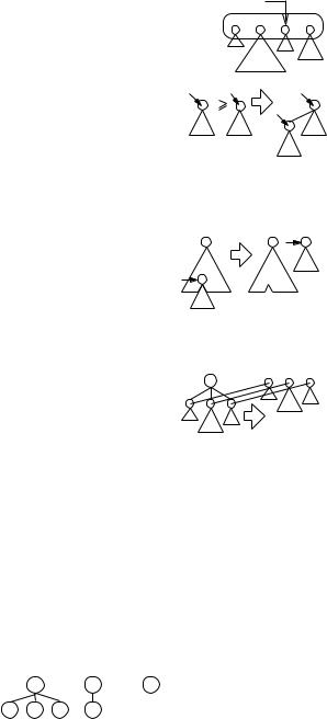
We shall discuss several variants of addressable priority queues. We start with the common principles underlying all of them. Figure 6.3 summarizes the commonalities.
In order to keep track of the current minimum, we maintain the handle to the root containing it. We use minPtr to denote this handle. The forest is manipulated using three simple operations: adding a new tree (and keeping minPtr up to date), combining two trees into a single one, and cutting out a subtree, making it a tree of its own.
An insert adds a new single-node tree to the forest. So a sequence of n inserts into an initially empty heap will simply create n single-node trees. The cost of an insert is clearly O(1).
A deleteMin operation removes the node indicated by minPtr. This turns all children of the removed node into roots. We then scan the set of roots (old and new) to find the new minimum, a potentially very costly process. We also perform some rebalancing, i.e., we combine trees into larger ones. The details of this process distinguish different kinds of addressable priority queue and are the key to efficiency.
We turn now to decreaseKey(h, k) which decreases the key value at a handle h to k. Of course, k must not be larger than the old key stored with h. Decreasing the
134 |
6 Priority Queues |
|
|
Class Handle = Pointer to PQItem |
minPtr |
||
Class AddressablePQ |
|||
roots |
|||
|
minPtr : Handle |
// root that stores the minimum |
|
|
roots : Set of Handle |
// pointers to tree roots |
|
Function min return element stored at minPtr
Procedure link(a,b : Handle) assert a ≤ b
remove b from roots make a the parent of b
Procedure combine(a,b : Handle) assert a and b are tree roots
if a ≤ b then link(a, b) else link(b, a)
Procedure newTree(h : Handle) roots := roots {h}
if h < min then minPtr := h
Procedure cut(h : Handle)
remove the subtree rooted at h from its tree newTree(h)
Function insert(e : Element) : Handle
i:=a Handle for a new PQItem storing e newTree(i)
return i
Function deleteMin : Element
e:= the Element stored in minPtr
foreach child h of the root at minPtr do cut(h) dispose minPtr
perform some rebalancing and update minPtr return e
Procedure decreaseKey(h : Handle, k : Key) change the key of h to k
if h is not a root then
cut(h); possibly perform some rebalancing
Procedure remove(h : Handle) decreaseKey(h, −∞);
Procedure merge(o : AddressablePQ)
if minPtr > (o.minPtr) then minPtr := o.minPtr roots := roots o.roots
b |
a |
a |
b
//
h
// h
e
//
// uses combine
deleteMin
o.roots := 0/; possibly perform some rebalancing
Fig. 6.3. Addressable priority queues
1 |
4 |
0 |
5 3 8 7
Fig. 6.4. A heap-ordered forest representing the set {0, 1, 3, 4, 5, 7, 8}
6.2 Addressable Priority Queues |
135 |
key associated with h may destroy the heap property because h may now be smaller than its parent. In order to maintain the heap property, we cut the subtree rooted at h and turn h into a root. This sounds simple enough, but may create highly skewed trees. Therefore, some variants of addressable priority queues perform additional operations to keep the trees in shape.
The remaining operations are easy. We can remove an item from the queue by first decreasing its key so that it becomes the minimum item in the queue, and then perform a deleteMin. To merge a queue o into another queue we compute the union of roots and o.roots. To update minPtr, it suffices to compare the minima of the merged queues. If the root sets are represented by linked lists, and no additional balancing is done, a merge needs only constant time.
In the remainder of this section we shall discuss particular implementations of addressable priority queues.
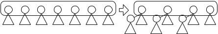
6.2.1 Pairing Heaps
Pairing heaps [67] use a very simple technique for rebalancing. Pairing heaps are efficient in practice; however a full theoretical analysis is missing. They rebalance only in deleteMin. If r1, . . . , rk is the sequence of root nodes stored in roots, then deleteMin combines r1 with r2, r3 with r4, etc., i.e., the roots are paired. Figure 6.5 gives an example.
roots |
|
|
|
g |
|
roots |
|
g |
|
b ≥ a |
c ≤ d |
f |
≥ e |
a |
c |
e |
|||
|
|
||||||||
|
|
|
|
b |
|
d |
f |
|
Fig. 6.5. The deleteMin operation for pairing heaps combines pairs of root nodes
Exercise 6.9 (three-pointer items). Explain how to implement pairing heaps using three pointers per heap item i: one to the oldest child (i.e., the child linked first to i), one to the next younger sibling (if any), and one to the next older sibling. If there is no older sibling, the third pointer goes to the parent. Figure 6.8 gives an example.
*Exercise 6.10 (two-pointer items). Explain how to implement pairing heaps using two pointers per heap item: one to the oldest child and one to next younger sibling. If there is no younger sibling, the second pointer goes to the parent. Figure 6.8 gives an example.
6.2.2 *Fibonacci Heaps
Fibonacci heaps [68] use more intensive balancing operations than do pairing heaps. This paves the way to a theoretical analysis. In particular, we obtain logarithmic

136 |
6 |
Priority Queues |
|
|
|
|
|
||
|
b |
c |
a |
|
d |
a |
feg e |
g |
a |
|
bac |
|
|
|
|
b |
|
f |
b |
b |
a c |
d |
f |
e g |
c d |
|
|
c d |
|
roots |
|
|
|
|
|
|
|
|
|
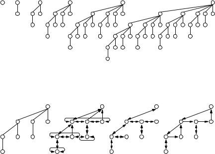
Fig. 6.6. An example of the development of the bucket array during execution of deleteMin for a Fibonacci heap. The arrows indicate the roots scanned. Note that scanning d leads to a cascade of three combine operations
amortized time for remove and deleteMin and worst-case constant time for all other operations.
Each item of a Fibonacci heap stores four pointers that identify its parent, one child, and two siblings (see Fig. 6.8). The children of each node form a doubly linked circular list using the sibling pointers. The sibling pointers of the root nodes can be used to represent roots in a similar way. Parent pointers of roots and child pointers of leaf nodes have a special value, for example, a null pointer.
In addition, every heap item contains a field rank. The rank of an item is the number of its children. In Fibonacci heaps, deleteMin links roots of equal rank r. The surviving root will then obtain a rank of r + 1. An efficient method to combine trees of equal rank is as follows. Let maxRank be an upper bound on the maximal rank of any node. We shall prove below that maxRank is logarithmic in n. Maintain a set of buckets, initially empty and numbered from 0 to maxRank. Then scan the list of old and new roots. When scanning a root of rank i, inspect the i-th bucket. If the i-th bucket is empty, then put the root there. If the bucket is nonempty, then combine the two trees into one. This empties the i-th bucket and creates a root of rank i + 1. Treat this root in the same way, i.e., try to throw it into the i + 1-th bucket. If it is occupied, combine . . . . When all roots have been processed in this way, we have a collection of trees whose roots have pairwise distinct ranks (see Figure 6.6).
A deleteMin can be very expensive if there are many roots. For example, a deleteMin following n insertions has a cost Ω(n). However, in an amortized sense, the cost of deletemin is O(maxRank). The reader must be familiar with the technique of amortized analysis (see Sect. 3.3) before proceeding further. For the amortized analysis, we postulate that each root holds one token. Tokens pay for a constant amount of computing time.
Lemma 6.2. The amortized complexity of deleteMin is O(maxRank).
Proof. A deleteMin first calls newTree at most maxRank times (since the degree of the old minimum is bounded by maxRank) and then initializes an array of size maxRank. Thus its running time is O(maxRank) and it needs to create maxRank new tokens. The remaining time is proportional to the number of combine operations performed. Each combine turns a root into a nonroot and is paid for by the token associated with the node turning into a nonroot.
6.2 Addressable Priority Queues |
137 |
How can we guarantee that maxRank stays small? Let us consider a simple situation first. Suppose that we perform a sequence of insertions followed by a one deleteMin. In this situation, we start with a certain number of single-node trees and all trees formed by combining are binomial trees, as shown in Fig. 6.7. The binomial tree B0 consists of a single node, and the binomial tree Bi+1 is obtained by combining two copies of Bi. This implies that the root of Bi has rank i and that Bi contains exactly 2i nodes. Thus the rank of a binomial tree is logarithmic in the size of the tree.
B0
B1
B2
B3
B4 |
B |
|
5 |
Fig. 6.7. The binomial trees of ranks zero to five
B3
|
3 pointers: |
|
4 pointers: |
pairing heaps, |
2 pointers: |
Fibonacci heaps |
binomial heaps |
Exercise 6.10 |
Fig. 6.8. Three ways to represent trees of nonuniform degree. The binomial tree of rank three, B3, is used as an example
Unfortunately, decreaseKey may destroy the nice structure of binomial trees. Suppose an item v is cut out. We now have to decrease the rank of its parent w. The problem is that the size of the subtrees rooted at the ancestors of w has decreased but their rank has not changed, and hence we can no longer claim that the size of a tree stays exponential in the rank of its root. Therefore, we have to perform some rebalancing to keep the trees in shape. An old solution [202] is to keep all trees in the heap binomial. However, this causes logarithmic cost for a decreaseKey.
*Exercise 6.11 (binomial heaps). Work out the details of this idea. Hint: cut the following links. For each ancestor of v and for v itself, cut the link to its parent. For
138 6 Priority Queues
1 |
|
|
1 |
6 |
3 |
|
,6) |
3 |
|
|
decreaseKey( |
|
||
9 |
8 |
9 |
|
|
5 |
|
|
5 |
|
7 |
|
|
7 |
|
decreaseKey( ,4)
4 1 6 7 5
3
4 1 6 7 5 2
decreaseKey( ,2)
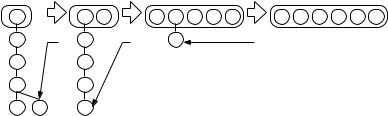
Fig. 6.9. An example of cascading cuts. Marks are drawn as crosses. Note that roots are never marked
each sibling of v of rank higher than v, cut the link to its parent. Argue that the trees stay binomial and that the cost of decreaseKey is logarithmic.
Fibonacci heaps allow the trees to go out of shape but in a controlled way. The idea is surprisingly simple and was inspired by the amortized analysis of binary counters (see Sect. 3.2.3). We introduce an additional flag for each node. A node may be marked or not. Roots are never marked. In particular, when newTree(h) is called in deleteMin, it removes the mark from h (if any). Thus when combine combines two trees into one, neither node is marked.
When a nonroot item x loses a child because decreaseKey has been applied to the child, x is marked; this assumes that x is not already marked. Otherwise, when x was already marked, we cut x, remove the mark from x, and attempt to mark x’s parent. If x’s parent is already marked, then . . . . This technique is called cascading cuts. In other words, suppose that we apply decreaseKey to an item v and that the k nearest ancestors of v are marked. We turn v and the k nearest ancestors of v into roots, unmark them, and mark the k + 1-th nearest ancestor of v (if it is not a root). Figure 6.9 gives an example. Observe the similarity to carry propagation in binary addition.
For the amortized analysis, we postulate that each marked node holds two tokens and each root holds one token. Please check that this assumption does not invalidate the proof of Lemma 6.2.
Lemma 6.3. The amortized complexity of decreaseKey is constant.
Proof. Assume that we decrease the key of item v and that the k nearest ancestors of v are marked. Here, k ≥ 0. The running time of the operation is O(1 + k). Each of the k marked ancestors carries two tokens, i.e., we have a total of 2k tokens available. We create k + 1 new roots and need one token for each of them. Also, we mark one unmarked node and need two tokens for it. Thus we need a total of k + 3 tokens. In other words, k − 3 tokens are freed. They pay for all but O(1) of the cost of decreaseKey. Thus the amortized cost of decreaseKey is constant.
How do cascading cuts affect the size of trees? We shall show that it stays exponential in the rank of the root. In order to do so, we need some notation. Recall
6.3 *External Memory |
139 |
the sequence 0, 1, 1, 2, 3, 5, 8, . . . of Fibonacci numbers. These are defined by the
recurrence F0 = 0, F1 = 1, and Fi = Fi−1 + Fi−2 |
for i ≥ 2. It is well known that |
|||||||||||
√ |
|
i |
i |
for all i |
≥ 0. |
|
|
|
|
|
||
Fi+1 ≥ ((1 + |
5)/2) ≥ 1.618 |
|
|
|
|
|
|
|||||
Exercise 6.12. Prove that Fi+2 ≥ ((1 + |
√ |
|
|
i |
≥ 1.618 |
i |
for all i ≥ 0 by induction. |
|||||
|
||||||||||||
5)/2) |
|
|
||||||||||
Lemma 6.4. Let v be any item in a Fibonacci heap and let i be the rank of v. The subtree rooted at v then contains at least Fi+2 nodes. In a Fibonacci heap with n items, all ranks are bounded by 1.4404 log n.
Proof. Consider an arbitrary item v of rank i. Order the children of v by the time at which they were made children of v. Let w j be the j-th child, 1 ≤ j ≤ i. When w j was made a child of v, both nodes had the same rank. Also, since at least the nodes w1, . . . , w j−1 were children of v at that time, the rank of v was at least j −1 then. The rank of w j has decreased by at most 1 since then, because otherwise w j would no longer be a child of v. Thus the current rank of w j is at least j − 2.
We can now set up a recurrence for the minimal number Si of nodes in a tree whose root has rank i. Clearly, S0 = 1, S1 = 2, and Si ≥ 2 + S0 + S1 + ··· + Si−2. The latter inequality follows from the fact that for j ≥ 2, the number of nodes in the subtree with root w j is at least S j−2, and that we can also count the nodes v and w1. The recurrence above (with = instead of ≥) generates the sequence 1, 2, 3, 5, 8,
. . . which is identical to the Fibonacci sequence (minus its first two elements).
Let us verify this by induction. Let T0 = 1, T1 = 2, and Ti = 2 + T0 + ··· + Ti−2 for i ≥ 2. Then, for i ≥ 2, Ti+1 − Ti = 2 + T0 + ··· + Ti−1 − 2 − T0 − ··· − Ti−2 = Ti−1,
i.e., Ti+1 = Ti + Ti−1. This proves Ti = Fi+2. |
√ |
|
|
For the second claim, we observe that Fi+2 ≤ n implies i · log((1 + |
|
5)/2) ≤ |
|
log n, which in turn implies i ≤ 1.4404 log n. |
|
||
This concludes our treatment of Fibonacci heaps. We have shown the following result.
Theorem 6.5. The following time bounds hold for Fibonacci heaps: min, insert, and merge take worst-case constant time; decreaseKey takes amortized constant time, and remove and deleteMin take an amortized time logarithmic in the size of the queue.
Exercise 6.13. Describe a variant of Fibonacci heaps where all roots have distinct ranks.
6.3 *External Memory
We now go back to nonaddressable priority queues and consider their cache efficiency and I/O efficiency. A weakness of binary heaps is that the siftDown operation goes down the tree in an unpredictable fashion. This leads to many cache faults and makes binary heaps prohibitively slow when they do not fit into the main memory.
140 6 Priority Queues
We now outline a data structure for (nonadressable) priority queues with more regular memory accesses. It is also a good example of a generally useful design principle: construction of a data structure out of simpler, known components and algorithms.
In this case, the components are internal-memory priority queues, sorting, and multiway merging (see also Sect. 5.7.1). Figure 6.10 depicts the basic design. The data structure consists of two priority queues Q and Q (e.g., binary heaps) and k sorted sequences S1, . . . , Sk. Each element of the priority queue is stored either in the insertion queue Q, in the deletion queue Q , or in one of the sorted sequences. The size of Q is limited to a parameter m. The deletion queue Q stores the smallest element of each sequence, together with the index of the sequence holding the element.
New elements are inserted into the insertion queue. If the insertion queue is full, it is first emptied. In this case, its elements form a new sorted sequence:
Procedure insert(e : Element) if |Q| = m then
k++; Sk := sort(Q); Q := 0/; Q .insert((Sk.popFront, k)) Q.insert(e)
The minimum is stored either in Q or in Q . If the minimum is in Q and comes from sequence Si, the next largest element of Si is inserted into Q :
Function deleteMin |
|
// assume min 0/ = ∞ |
|
if min Q ≤ min Q then e := Q.deleteMin |
|||
else (e, i) := Q .deleteMin |
|
||
|
|
then Q .insert((Si.popFront, i)) |
|
if Si = |
|
|
|
return e
It remains to explain how the ingredients of our data structure are mapped to the memory hierarchy. The queues Q and Q are stored in internal memory. The size bound m for Q should be a constant fraction of the internal-memory size M and a multiple of the block size B. The sequences Si are largely kept externally. Initially, only the B smallest elements of Si are kept in an internal-memory buffer bi. When the last element of bi is removed, the next B elements of Si are loaded. Note that we are effectively merging the sequences Si. This is similar to our multiway merging
S1
external 
 B
B 

S2 Sk
insert
... Q
sort
Q
m
 min
min 
Fig. 6.10. Schematic view of an external-memory priority queue
6.4 Implementation Notes |
141 |
algorithm described in Sect. 5.7.1. Each inserted element is written to disk at most once and fetched back to internal memory at most once. Since all disk accesses are in units of at least a full block, the I/O requirement of our algorithm is at most n/B for n queue operations.
Our total requirement for internal memory is at most m + kB + 2k. This is below the total fast-memory size M if m = M/2 and k ≤ (M/2 − 2k)/B ≈ M/(2B). If there are many insertions, the internal memory may eventually overflow. However, the earliest this can happen is after m(1 + (M/2 − 2k)/B ) ≈ M2/(4B) insertions. For example, if we have 1 Gbyte of main memory, 8-byte elements, and 512 Kbyte disk blocks, we have M = 227 and B = 216 (measured in elements). We can then perform about 236 insertions – enough for 128 Gbyte of data. Similarly to external mergesort, we can handle larger amounts of data by performing multiple phases of multiway merging (see, [31, 164]). The data structure becomes considerably more complicated, but it turns out that the I/O requirement for n insertions and deletions is about the same as for sorting n elements. An implementation of this idea is two to three times faster than binary heaps for the hierarchy between cache and main memory [164]. There are also implementations for external memory [48].
6.4 Implementation Notes
There are various places where sentinels (see Chap. 3) can be used to simplify or (slightly) accelerate the implementation of priority queues. Since sentinels may require additional knowledge about key values, this could make a reusable implementation more difficult, however.
•If h[0] stores a Key no larger than any Key ever inserted into a binary heap, then siftUp need not treat the case i = 1 in a special way.
•If h[n + 1] stores a Key no smaller than any Key ever inserted into a binary heap, then siftDown need not treat the case 2i + 1 > n in a special way. If such large keys are stored in h[n + 1..2n + 1], then the case 2i > n can also be eliminated.
•Addressable priority queues can use a special dummy item rather than a null pointer.
For simplicity we have formulated the operations siftDown and siftUp for binary heaps using recursion. It might be a little faster to implement them iteratively instead. Similarly, the swap operations could be replaced by unidirectional move operations thus halving the number of memory accesses.
Exercise 6.14. Give iterative versions of siftDown and siftUp. Also replace the swap operations.
Some compilers do the recursion elimination for you.
As for sequences, memory management for items of addressable priority queues can be critical for performance. Often, a particular application may be able to do this more efficiently than a general-purpose library. For example, many graph algorithms use a priority queue of nodes. In this case, items can be incorporated into nodes.