

Algorithms and data structures
.pdf40 2 Introduction
KaratsubaÕs algorithm, is not covered by our master theorem, which neglects rounding issues. We shall now show how to extend the master theorem to the following recurrence:
|
if n ≤ n0, |
r(n) ≤ a |
cn + d · r( n/b + e) if n > n0,
where a, b, c, d, and e are constants, and n0 is such that n/b + e < n for n > n0. We proceed in two steps. We Þrst concentrate on n of the form bk + z, where z is such that
z/b + e = z. For example, for b = 2 and e = 3, we would choose z = 6. Note that for n of this form, we have n/b + e = (bk + z)/b + e = bk−1 + z/b + e = bk−1 + z,
i.e., the reduced problem size has the same form. For the nÕs in this special form, we then argue exactly as in Theorem 2.5.
How do we generalize to arbitrary n? The simplest way is semantic reasoning. It is clear4 that the cost grows with the problem size, and hence the cost for an input of size n will be no larger than the cost for an input whose size is equal to the next input size of special form. Since this input is at most b times larger and b is a constant, the bound derived for special n is affected only by a constant factor.
The formal reasoning is as follows (you may want to skip this paragraph and come back to it when the need arises). We deÞne a function R(n) by the same recurrence, with ≤ replaced by equality: R(n) = a for n ≤ n0 and R(n) = cn + dR( n/b + e) for n > n0. Obviously, r(n) ≤ R(n). We derive a bound for R(n) and n of special form as described above. Finally, we argue by induction that R(n) ≤ R(s(n)), where s(n) is the smallest number of the form bk + z with bk + z ≥ n. The induction step is as follows:
R(n) = cn + dR( n/b + e) ≤ cs(n) + dR(s( n/b + e)) = R(s(n)) ,
where the inequality uses the induction hypothesis and n ≤ s(n). The last equality uses the fact that for s(n) = bk + z (and hence bk−1 + z < n), we have bk−2 + z <
n/b + e ≤ bk−1 + z and hence s( n/b + e) = bk−1 + z = s(n)/b + e.
There are many generalizations of the master theorem: we might break the recursion earlier, the cost for dividing and conquering may be nonlinear, the size of the subproblems might vary within certain bounds, the number of subproblems may depend on the input size, etc. We refer the reader to the books [81, 175] for further information.
Exercise 2.8. Consider the recurrence |
|
1 |
if n = 1, |
C(n) = |
|
C( n/2 ) + C( n/2 ) + cn if n > 1.
Show that C(n) = O(n log n).
4Be aware that most errors in mathematical arguments are near occurrences of the word ÒclearlyÓ.
2.7 Average-Case Analysis |
41 |
*Exercise 2.9. Suppose you have a divide-and-conquer algorithm whose running
|
|
|
|
|
|
|
|
|
|
|
|
|
|
|
( ) = |
a, T |
( |
n |
) = |
cn |
+ |
√n |
|
T |
( |
/ |
|
) |
|
time is governed by the recurrence T 1 |
|
|
|
|
n |
√n |
. |
|||||||
Show that the running time of the program is O(n log log n).
Exercise 2.10. Access to data structures is often governed by the following recurrence: T (1) = a, T (n) = c + T (n/2). Show that T (n) = O(log n).
2.6.3 Global Arguments
The algorithm analysis techniques introduced so far are syntax-oriented in the following sense: in order to analyze a large program, we Þrst analyze its parts and then combine the analyses of the parts into an analysis of the large program. The combination step involves sums and recurrences.
We shall also use a completely different approach which one might call semanticsoriented. In this approach we associate parts of the execution with parts of a combinatorial structure and then argue about the combinatorial structure. For example, we might argue that a certain piece of program is executed at most once for each edge of a graph or that the execution of a certain piece of program at least doubles the size of a certain structure, that the size is one initially, and at most n at termination, and hence the number of executions is bounded logarithmically.
2.7 Average-Case Analysis
In this section we shall introduce you to average-case analysis. We shall do so by way of three examples of increasing complexity. We assume that you are familiar with basic concepts of probability theory such as discrete probability distributions, expected values, indicator variables, and the linearity of expectations. Section A.3 reviews the basics.
2.7.1 Incrementing a Counter
We begin with a very simple example. Our input is an array a[0..n − 1] Þlled with digits zero and one. We want to increment the number represented by the array by one.
i := 0
while (i < n and a[i] = 1) do a[i] = 0; i++; if i < n then a[i] = 1
How often is the body of the while loop executed? Clearly, n times in the worst case and 0 times in the best case. What is the average case? The Þrst step in an average-case analysis is always to deÞne the model of randomness, i.e., to deÞne the underlying probability space. We postulate the following model of randomness: each digit is zero or one with probability 1/2, and different digits are independent. The loop body is executed k times, 0 ≤ k ≤ n, iff the last k + 1 digits of a are 01k or k
42 2 Introduction
is equal to n and all digits of a are equal to one. The former event has probability 2−(k+1), and the latter event has probability 2−n. Therefore, the average number of executions is equal to
∑ k2−(k+1) + n2−n ≤ ∑ k2−k = 2 ,
0≤k<n k≥0
where the last equality is the same as (A.14).
2.7.2 Left-to-Right Maxima
Our second example is slightly more demanding. Consider the following simple program that determines the maximum element in an array a[1..n]:
m := a[1]; for i := 2 to n do if a[i] > m then m := a[i]
How often is the assignment m := a[i] executed? In the worst case, it is executed in every iteration of the loop and hence n − 1 times. In the best case, it is not executed at all. What is the average case? Again, we start by deÞning the probability space. We assume that the array contains n distinct elements and that any order of these elements is equally likely. In other words, our probability space consists of the n! permutations of the array elements. Each permutation is equally likely and therefore has probability 1/n!. Since the exact nature of the array elements is unimportant, we may assume that the array contains the numbers 1 to n in some order. We are interested in the average number of left-to-right maxima. A left-to-right maximum in a sequence is an element which is larger than all preceding elements. So, (1, 2, 4, 3) has three left-to-right-maxima and (3, 1, 2, 4) has two left-to-right-maxima. For a permutation π of the integers 1 to n, let Mn(π ) be the number of left-to-right-maxima. What is E[Mn]? We shall describe two ways to determine the expectation. For small n, it is easy to determine E[Mn] by direct calculation. For n = 1, there is only one permutation, namely (1), and it has one maximum. So E[M1] = 1. For n = 2, there are two permutations, namely (1, 2) and (2, 1). The former has two maxima and the latter has one maximum. So E[M2] = 1.5. For larger n, we argue as follows.
We write Mn as a sum of indicator variables I1 to In, i.e., Mn = I1 + . . . + In, where Ik is equal to one for a permutation π if the k-th element of π is a left-to-right maximum. For example, I3((3, 1, 2, 4)) = 0 and I4((3, 1, 2, 4)) = 1. We have
E[Mn] = E[I1 + I2 + . . . + In]
=E[I1] + E[I2] + . . . + E[In]
=prob(I1 = 1) + prob(I2 = 1) + . . . + prob(In = 1) ,
where the second equality is the linearity of expectations (A.2) and the third equality follows from the IkÕs being indicator variables. It remains to determine the probability that Ik = 1. The k-th element of a random permutation is a left-to-right maximum if and only if the k-th element is the largest of the Þrst k elements. In a random permutation, any position is equally likely to hold the maximum, so that the probability we are looking for is prob(Ik = 1) = 1/k and hence
2.7 Average-Case Analysis |
43 |
E[Mn] = ∑ prob(Ik = 1) = |
∑ |
1 |
. |
|
|||
1≤k≤n |
1≤k≤n |
k |
|
|
|
||
So, E[M4] = 1+ 1/2+ 1/3+ 1/4 = (12+ 6+ 4+ 3)/12 = 25/12. The sum ∑1≤k≤n 1/k will appear several times in this book. It is known under the name Òn-th harmonic
numberÓ and is denoted by Hn. It is known that ln n ≤ Hn ≤ 1 + ln n, i.e., Hn ≈ ln n; see (A.12). We conclude that the average number of left-to-right maxima is much smaller than in the worst case.
n |
1 |
n |
1 |
|
n 1 |
|
||
Exercise 2.11. Show that ∑ |
|
≤ ln n + 1. Hint: show Þrst that ∑ |
|
≤ |
|
|
dx. |
|
k |
k |
1 x |
||||||
k=1 |
|
|
k=2 |
|
|
|
|
|
We now describe an alternative analysis. We introduce An as a shorthand for E[Mn] and set A0 = 0. The Þrst element is always a left-to-right maximum, and each number is equally likely as the Þrst element. If the Þrst element is equal to i, then only the numbers i + 1 to n can be further left-to-right maxima. They appear in random order in the remaining sequence, and hence we shall see an expected number of An−i
further maxima. Thus |
|
|
|
An = 1 + ∑ An−i |
/n or nAn = n + ∑ Ai . |
1≤i≤n |
0≤i≤n−1 |
A simple trick simpliÞes this recurrence. The corresponding equation for n − 1 instead of n is (n − 1)An−1 = n − 1 + ∑1≤i≤n−2 Ai. Subtracting the equation for n − 1 from the equation for n yields
nAn − (n − 1)An−1 = 1 + An−1 or An = 1/n + An−1 ,
and hence An = Hn.
2.7.3 Linear Search
We come now to our third example; this example is even more demanding. Consider the following search problem. We have items 1 to n, which we are required to arrange linearly in some order; say, we put item i in position i. Once we have arranged the items, we perform searches. In order to search for an item x, we go through the sequence from left to right until we encounter x. In this way, it will take i steps to access item i.
Suppose now that we also know that we shall access the items with different probabilities; say, we search for item i with probability pi, where pi ≥ 0 for all i, 1 ≤ i ≤ n, and ∑i pi = 1. In this situation, the expected or average cost of a search is equal to ∑i pi i, since we search for item i with probability pi and the cost of the search is i.
What is the best way of arranging the items? Intuition tells us that we should arrange the items in order of decreasing probability. Let us prove this.
44 2 Introduction
Lemma 2.6. An arrangement is optimal with respect to the expected search cost if it has the property that pi > p j implies i < j. If p1 ≥ p2 ≥ . . . ≥ pn, the placementi = i results in the optimal expected search cost Opt = ∑i pii.
Proof. Consider an arrangement in which, for some i and j, we have pi > p j andi > j, i.e., item i is more probable than item j and yet placed after it. Interchanging items i and j changes the search cost by
−( pi i + p j j) + (pi j + p j i) = (pi − p j)( i − j) < 0 ,
i.e., the new arrangement is better and hence the old arrangement is not optimal. Let us now consider the case p1 > p2 > . . . > pn. Since there are only n! possible
arrangements, there is an optimal arrangement. Also, if i < j and i is placed after j, the arrangement is not optimal by the argument in the preceding paragraph. Thus the optimal arrangement puts item i in position i = i and its expected search cost is
∑i pii.
If p1 ≥ p2 ≥ . . . ≥ pn, the arrangement i = i for all i is still optimal. However, if some probabilities are equal, we have more than one optimal arrangement. Within blocks of equal probabilities, the order is irrelevant.
Can we still do something intelligent if the probabilities pi are not known to us? The answer is yes, and a very simple heuristic does the job. It is called the move-to- front heuristic. Suppose we access item i and Þnd it in position i. If i = 1, we are happy and do nothing. Otherwise, we place it in position 1 and move the items in positions 1 to i − 1 one position to the rear. The hope is that, in this way, frequently accessed items tend to stay near the front of the arrangement and infrequently accessed items move to the rear. We shall now analyze the expected behavior of the move-to-front heuristic.
Consider two items i and j and suppose that both of them were accessed in the past. Item i will be accessed before item j if the last access to item i occurred after the last access to item j. Thus the probability that item i is before item j is pi/( pi + p j). With probability p j/( pi + p j), item j stands before item i.
Now, i is simply one plus the number of elements before i in the list. Thus
the expected value of i is equal to 1 + ∑ j; |
j=i |
p j/( pi + p j), and hence the expected |
||||||||
search cost in the move-to-front heuristic is |
|
|
|
|
|
|
||||
|
|
|
p j |
|
|
|
pi p j |
|
||
CMTF = ∑ pi |
1 |
+ ∑ |
|
|
|
= ∑ pi + ∑ |
|
. |
||
pi + p j |
pi + p j |
|||||||||
i |
|
j; j=i |
i |
i, j; i= j |
|
|||||
|
|
|
|
|
|
|
|
|||
Observe that for each i and j with i = j, the term pi p j/( pi + p j) appears twice in the sum above. In order to proceed with the analysis, we assume p1 ≥ p2 ≥ . . . ≥ pn. This is an assumption used in the analysis, the algorithm has no knowledge of this. Then

2.8 Randomized Algorithms |
45 |
|
|
|
|
|
|
|
|
|
|
CMTF = ∑ pi |
+ 2 |
∑ |
|
pi p j |
= ∑ pi |
1 + 2 ∑ |
|
p j |
|
|
pi + p j |
pi |
+ p j |
||||||
i |
|
j; j<i |
i |
j; j<i |
|||||
|
|
|
|
|
|||||
|
|
|
|
|
|
|
|
||
≤ ∑ pi |
1 + 2 ∑ 1 |
< ∑ pi2i = 2 ∑ pii = 2Opt . |
|||||||
i |
|
|
j; j<i |
i |
i |
|
|
|
|
Theorem 2.7. The move-to-front heuristic achieves an expected search time which is at most twice the optimum.
2.8 Randomized Algorithms
Suppose you are offered the chance to participate in a TV game show. There are 100 boxes that you can open in an order of your choice. Box i contains an amount mi of money. This amount is unknown to you but becomes known once the box is opened. No two boxes contain the same amount of money. The rules of the game are very simple:
•At the beginning of the game, the presenter gives you 10 tokens.
•When you open a box and the contents of the box are larger than the contents of all previously opened boxes, you have to hand back a token.5
•When you have to hand back a token but have no tokens, the game ends and you lose.
•When you manage to open all of the boxes, you win and can keep all the money.
There are strange pictures on the boxes, and the presenter gives hints by suggesting the box to be opened next. Your aunt, who is addicted to this show, tells you that only a few candidates win. Now, you ask yourself whether it is worth participating in this game. Is there a strategy that gives you a good chance of winning? Are the presenterÕs hints useful?
Let us Þrst analyze the obvious algorithm Ð you always follow the presenter. The worst case is that he makes you open the boxes in order of increasing value. Whenever you open a box, you have to hand back a token, and when you open the 11th box you are dead. The candidates and viewers would hate the presenter and he would soon be Þred. Worst-case analysis does not give us the right information in this situation. The best case is that the presenter immediately tells you the best box. You would be happy, but there would be no time to place advertisements, so that the presenter would again be Þred. Best-case analysis also does not give us the right information in this situation. We next observe that the game is really the left-to- right maxima question of the preceding section in disguise. You have to hand back a token whenever a new maximum shows up. We saw in the preceding section that the expected number of left-to-right maxima in a random permutation is Hn, the n-th
5The contents of the Þrst box opened are larger than the contents of all previously opened boxes, and hence the Þrst token goes back to the presenter in the Þrst round.
46 2 Introduction
harmonic number. For n = 100, Hn < 6. So if the presenter were to point to the boxes in random order, you would have to hand back only 6 tokens on average. But why should the presenter offer you the boxes in random order? He has no incentive to have too many winners.
The solution is to take your fate into your own hands: open the boxes in random order. You select one of the boxes at random, open it, then choose a random box from the remaining ones, and so on. How do you choose a random box? When there are k boxes left, you choose a random box by tossing a die with k sides or by choosing a random number in the range 1 to k. In this way, you generate a random permutation of the boxes and hence the analysis in the previous section still applies. On average you will have to return fewer than 6 tokens and hence your 10 tokens sufÞce. You have just seen a randomized algorithm. We want to stress that, although the mathematical analysis is the same, the conclusions are very different. In the average-case scenario, you are at the mercy of the presenter. If he opens the boxes in random order, the analysis applies; if he does not, it does not. You have no way to tell, except after many shows and with hindsight. In other words, the presenter controls the dice and it is up to him whether he uses fair dice. The situation is completely different in the randomized-algorithms scenario. You control the dice, and you generate the random permutation. The analysis is valid no matter what the presenter does.
2.8.1 The Formal Model
Formally, we equip our RAM with an additional instruction: Ri := randInt(C) assigns a random integer between 0 and C −1 to Ri. In pseudocode, we write v:= randInt(C), where v is an integer variable. The cost of making a random choice is one time unit. Algorithms not using randomization are called deterministic.
The running time of a randomized algorithm will generally depend on the random choices made by the algorithm. So the running time on an instance i is no longer a number, but a random variable depending on the random choices. We may eliminate the dependency of the running time on random choices by equipping our machine with a timer. At the beginning of the execution, we set the timer to a value T (n), which may depend on the size n of the problem instance, and stop the machine once the timer goes off. In this way, we can guarantee that the running time is bounded by T (n). However, if the algorithm runs out of time, it does not deliver an answer.
The output of a randomized algorithm may also depend on the random choices made. How can an algorithm be useful if the answer on an instance i may depend on the random choices made by the algorithm Ð if the answer may be ÒYesÓ today and ÒNoÓ tomorrow? If the two cases are equally probable, the answer given by the algorithm has no value. However, if the correct answer is much more likely than the incorrect answer, the answer does have value. Let us see an example.
Alice and Bob are connected over a slow telephone line. Alice has an integer xA and Bob has an integer xB, each with n bits. They want to determine whether they have the same number. As communication is slow, their goal is to minimize the amount of information exchanged. Local computation is not an issue.

2.8 Randomized Algorithms |
47 |
In the obvious solution, Alice sends her number to Bob, and Bob checks whether the numbers are equal and announces the result. This requires them to transmit n digits. Alternatively, Alice could send the number digit by digit, and Bob would check for equality as the digits arrived and announce the result as soon as he knew it, i.e., as soon as corresponding digits differed or all digits had been transmitted. In the worst case, all n digits have to be transmitted. We shall now show that randomization leads to a dramatic improvement. After transmission of only O(log n) bits, equality and inequality can be decided with high probability.
Alice and Bob follow the following protocol. Each of them prepares an ordered list of prime numbers. The list consists of the smallest L primes with k or more bits and leading bit 1. Each such prime has a value of at least 2k. We shall say more about the choice of L and k below. In this way, it is guaranteed that both Alice and Bob generate the same list. Then Alice chooses an index i, 1 ≤ i ≤ L, at random and sends i and xA mod pi to Bob. Bob computes xB mod pi. If xA mod pi = xB mod pi, he declares that the numbers are different. Otherwise, he declares the numbers the same. Clearly, if the numbers are the same, Bob will say so. If the numbers are different and xA mod pi = xB mod pi, he will declare them different. However, if xA = xB and yet xA mod pi = xB mod pi, he will erroneously declare the numbers equal. What is the probability of an error?
An error occurs if xA = xB but xA ≡ xB( mod pi). The latter condition is equivalent to pi dividing the difference D = xA − xB. This difference is at most 2n in absolute value. Since each prime pi has a value of at least 2k, our list contains at most n/k primes that divide6 the difference, and hence the probability of error is at most (n/k)/L. We can make this probability arbitrarily small by choosing L large enough. If, say, we want to make the probability less than 0.000001 = 10−6, we choose L = 106(n/k).
What is the appropriate choice of k? Out of the numbers with k bits, approximately 2k/k are primes.7 Hence, if 2k/k ≥ 106n/k, the list will contain only k-bit integers. The condition 2k ≥ 106n is tantamount to k ≥ log n + 6 log 10. With this choice of k, the protocol transmits log L + k = log n + 12 log 10 bits. This is exponentially better than the naive protocol.
What can we do if we want an error probability less than 10−12? We could redo the calculations above with L = 1012n. Alternatively, we could run the protocol twice and declare the numbers different if at least one run declares them different. This
two-stage protocol errs only if both runs err, and hence the probability of error is at most 10−6 · 10−6 = 10−12.
Exercise 2.12. Compare the efÞciency of the two approaches for obtaining an error probability of 10−12.
6Let d be the number of primes on our list that divide D. Then 2n ≥ |D| ≥ (2k)d = 2kd and hence d ≤ n/k.
7For any integer x, let π (x) be the number of primes less than or equal to x. For example, π (10) = 4 because there are four prime numbers (2, 3, 5 and 7) less than or equal to 10. Then x/(ln x + 2) < π (x) < x/(ln x − 4) for x ≥ 55. See the Wikipedia entry on Òprime numbersÓ for more information.
48 2 Introduction
Exercise 2.13. In the protocol described above, Alice and Bob have to prepare ridiculously long lists of prime numbers. Discuss the following modiÞed protocol. Alice chooses a random k-bit integer p (with leading bit 1) and tests it for primality. If p is not prime, she repeats the process. If p is prime, she sends p and xA mod p to Bob.
Exercise 2.14. Assume you have an algorithm which errs with a probability of at most 1/4 and that you run the algorithm k times and output the majority output. Derive a bound on the error probability as a function of k. Do a precise calculation for k = 2 and k = 3, and give a bound for large k. Finally, determine k such that the error probability is less than a given ε .
2.8.2 Las Vegas and Monte Carlo Algorithms
Randomized algorithms come in two main varieties, the Las Vegas and the Monte Carlo variety. A Las Vegas algorithm always computes the correct answer but its running time is a random variable. Our solution for the game show is a Las Vegas algorithm; it always Þnds the box containing the maximum; however, the number of left-to-right maxima is a random variable. A Monte Carlo algorithm always has the same run time, but there is a nonzero probability that it gives an incorrect answer. The probability that the answer is incorrect is at most 1/4. Our algorithm for comparing two numbers over a telephone line is a Monte Carlo algorithm. In Exercise 2.14, it is shown that the error probability can be made arbitrarily small.
Exercise 2.15. Suppose you have a Las Vegas algorithm with an expected execution time t(n), and that you run it for 4t(n) steps. If it returns an answer within the alloted time, this answer is returned, otherwise an arbitrary answer is returned. Show that the resulting algorithm is a Monte Carlo algorithm.
Exercise 2.16. Suppose you have a Monte Carlo algorithm with an execution time m(n) that gives a correct answer with probability p and a deterministic algorithm that veriÞes in time v(n) whether the Monte Carlo algorithm has given the correct answer. Explain how to use these two algorithms to obtain a Las Vegas algorithm with expected execution time (m(n) + v(n))/(1 − p).
We come back to our game show example. You have 10 tokens available to you. The expected number of tokens required is less than 6. How sure should you be that you will go home a winner? We need to bound the probability that Mn is larger than 11, because you lose exactly if the sequence in which you order the boxes has 11 or more left-to-right maxima. Markov’s inequality allows you to bound this probability. It states that, for a nonnegative random variable X and any constant c ≥ 1, prob(X ≥ c · E[X])≤ 1/c; see (A.4) for additional information. We apply the inequality with X = Mn and c = 11/6. We obtain
|
|
11 |
E[Mn] |
|
6 |
|
prob(Mn ≥ 11) ≤ prob |
Mn ≥ |
|
≤ |
|
, |
|
6 |
11 |
and hence the probability of winning is more than 5/11.
2.9 Graphs |
49 |
2.9 Graphs
Graphs are an extremely useful concept in algorithmics. We use them whenever we want to model objects and relations between them; in graph terminology, the objects are called nodes, and the relations between nodes are called edges. Some obvious applications are road maps and communication networks, but there are also more abstract applications. For example, nodes could be tasks to be completed when building a house, such as Òbuild the wallsÓ or Òput in the windowsÓ, and edges could model precedence relations such as Òthe walls have to be built before the windows can be put inÓ. We shall also see many examples of data structures where it is natural to view objects as nodes and pointers as edges between the object storing the pointer and the object pointed to.
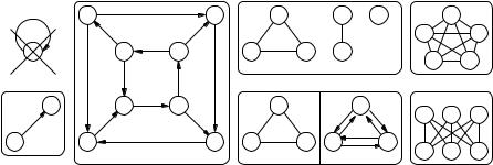
When humans think about graphs, they usually Þnd it convenient to work with pictures showing nodes as bullets and edges as lines and arrows. To treat graphs algorithmically, a more mathematical notation is needed: a directed graph G = (V, E) is a pair consisting of a node set (or vertex set) V and an edge set (or arc set) E V ×V . We sometimes abbreviate Òdirected graphÓ to digraph. For example, Fig. 2.7 shows the graph G = ({s, t, u, v, w, x, y, z}, {(s, t), (t, u), (u, v), (v, w), (w, x), (x, y), (y, z), (z, s),
(s, v), (z, w), (y, t), (x, u)}). Throughout this book, we use the convention n = |V | and m = |E| if no other deÞnitions for n or m are given. An edge e = (u, v) E represents a connection from u to v. We call u and v the source and target, respectively, of e. We say that e is incident on u and v and that v and u are adjacent. The special case of a self-loop (v, v) is disallowed unless speciÞcally mentioned.
The outdegree of a node v is the number of edges leaving it, and its indegree is the number of edges ending at it, formally, outdegree(v) = |{(v, u) E}| and indegree(v) = |{(u, v) E}|. For example, node w in graph G in Fig. 2.7 has indegree two and outdegree one.
A bidirected graph is a digraph where, for any edge (u, v), the reverse edge (v, u) is also present. An undirected graph can be viewed as a streamlined representation of a bidirected graph, where we write a pair of edges (u, v), (v, u) as the two-element set {u, v}. Figure 2.7 shows a three-node undirected graph and its bidirected counterpart. Most graph-theoretic terms for undirected graphs have the same deÞnition as for
self−loop |
s |
|
1 |
t |
|
u |
s |
x |
K5 |
|
|
|
|
1 |
2 |
|
|
|
|
|
|
|
|
|
|
|
|
|
|
|
||
|
|
|
z |
y |
|
w |
v |
t |
|
|
|
|
|
|
1 |
|
|
|
U |
|
|
|
|
2 |
−2 |
1 |
1 |
|
|
|
|
|
H |
w |
|
w |
1 |
|
|
u |
u |
|
K3,3 |
|
x |
|
|
|
||||||
|
1 |
|
1 |
1 |
2 |
|
|
|
|
|
v |
|
v |
|
u |
w |
v |
w |
v |
|
|
|
|
|
|
|||||||
|
|
|
|
G |
|
undirected |
bidirected |
|
||
Fig. 2.7. Some graphs