

Algorithms and data structures
.pdfXII |
Contents |
|
References . . . . . . . . . . . . . . . . . . . . . . . . . . . . . . . . . . . . . . . . . . . . . . . . . . . . . . . . . |
273 |
|
Index . |
. . . . . . . . . . . . . . . . . . . . . . . . . . . . . . . . . . . . . . . . . . . . . . . . . . . . . . . . . . . . |
285 |
1
Appetizer: Integer Arithmetics
An appetizer is supposed to stimulate the appetite at the beginning of a meal. This is exactly the purpose of this chapter. We want to stimulate your interest in algorithmic1 techniques by showing you a surprising result. The school method for multiplying integers is not the best multiplication algorithm; there are much faster ways to multiply large integers, i.e., integers with thousands or even millions of digits, and we shall teach you one of them.
Arithmetic on long integers is needed in areas such as cryptography, geometric computing, and computer algebra and so an improved multiplication algorithm is not just an intellectual gem but also useful for applications. On the way, we shall learn basic analysis and basic algorithm engineering techniques in a simple setting. We shall also see the interplay of theory and experiment.
We assume that integers are represented as digit strings. In the base B number system, where B is an integer larger than one, there are digits 0, 1, to B − 1 and a digit string an−1an−2 . . . a1a0 represents the number ∑0≤i<n aiBi. The most important systems with a small value of B are base 2, with digits 0 and 1, base 10, with digits 0 to 9, and base 16, with digits 0 to 15 (frequently written as 0 to 9, A, B, C, D, E, and F). Larger bases, such as 28, 216, 232, and 264, are also useful. For example,
“10101” |
in base 2 represents |
1 · 24 + 0 · 23 + 1 · 22 + 0 · 21 + 1 · 20 |
= |
21, |
“924” |
in base 10 represents |
9 · 102 + 2 · 101 + 4 · 100 |
= |
924 . |
We assume that we have two primitive operations at our disposal: the addition of three digits with a two-digit result (this is sometimes called a full adder), and the
1The Soviet stamp on this page shows Muhammad ibn Musa al-Khwarizmi (born approximately 780; died between 835 and 850), Persian mathematician and astronomer from the Khorasan province of present-day Uzbekistan. The word “algorithm” is derived from his name.
2 1 Appetizer: Integer Arithmetics
multiplication of two digits with a two-digit result.2 For example, in base 10, we
have
3
5
and 6 · 7 = 42 .
5
13
We shall measure the efficiency of our algorithms by the number of primitive operations executed.
We can artificially turn any n-digit integer into an m-digit integer for any m ≥ n by adding additional leading zeros. Concretely, “425” and “000425” represent the same integer. We shall use a and b for the two operands of an addition or multiplication and assume throughout this section that a and b are n-digit integers. The assumption that both operands have the same length simplifies the presentation without changing the key message of the chapter. We shall come back to this remark at the end of the chapter. We refer to the digits of a as an−1 to a0, with an−1 being the most significant digit (also called leading digit) and a0 being the least significant digit, and write a = (an−1 . . . a0). The leading digit may be zero. Similarly, we use bn−1 to b0 to denote the digits of b, and write b = (bn−1 . . . b0).
1.1 Addition
We all know how to add two integers a = (an−1 . . . a0) and b = (bn−1 . . . b0). We simply write one under the other with the least significant digits aligned, and sum the integers digitwise, carrying a single digit from one position to the next. This digit is called a carry. The result will be an n + 1-digit integer s = (sn . . . s0). Graphically,
|
an−1 |
. . . a1 |
a0 |
first operand |
|
bn−1 |
. . . b1 |
b0 |
second operand |
cn |
cn−1 |
. . . c1 |
0 |
carries |
sn |
sn−1 |
. . . s1 |
s0 |
sum |
where cn to c0 is the sequence of carries and s = (sn . . . s0) is the sum. We have c0 = 0, ci+1 · B + si = ai + bi + ci for 0 ≤ i < n and sn = cn. As a program, this is written as
c = 0 : Digit |
// Variable for the carry digit |
for i := 0 to n − 1 do |
add ai, bi, and c to form si and a new carry c |
sn := c |
|
We need one primitive operation for each position, and hence a total of n primitive operations.
Theorem 1.1. The addition of two n-digit integers requires exactly n primitive operations. The result is an n + 1-digit integer.
2Observe that the sum of three digits is at most 3(B − 1) and the product of two digits is at most (B−1)2, and that both expressions are bounded by (B−1) ·B1 + (B−1) ·B0 = B2 −1, the largest integer that can be written with two digits.

1.2 Multiplication: The School Method |
3 |
1.2 Multiplication: The School Method
We all know how to multiply two integers. In this section, we shall review the “school method”. In a later section, we shall get to know a method which is significantly faster for large integers.
We shall proceed slowly. We first review how to multiply an n-digit integer a by a one-digit integer b j. We use b j for the one-digit integer, since this is how we need it below. For any digit ai of a, we form the product ai · b j. The result is a two-digit integer (cidi), i.e.,
ai · b j = ci · B + di .
We form two integers, c = (cn−1 . . . c0 0) and d = (dn−1 . . . d0), from the c’s and d’s, respectively. Since the c’s are the higher-order digits in the products, we add a zero digit at the end. We add c and d to obtain the product p j = a · b j. Graphically,
(an−1 . . . ai . . . a0) · b j −→ |
cn−1 cn−2 . . . ci ci−1 . . . c0 0 |
dn−1 . . . di+1 di . . . d1 d0 |
|
|
sum of c and d |
Let us determine the number of primitive operations. For each i, we need one primitive operation to form the product ai · b j, for a total of n primitive operations. Then we add two n + 1-digit numbers. This requires n + 1 primitive operations. So the total number of primitive operations is 2n + 1.
Lemma 1.2. We can multiply an n-digit number by a one-digit number with 2n + 1 primitive operations. The result is an n + 1-digit number.
When you multiply an n-digit number by a one-digit number, you will probably proceed slightly differently. You combine3 the generation of the products ai ·b j with the summation of c and d into a single phase, i.e., you create the digits of c and d when they are needed in the final addition. We have chosen to generate them in a separate phase because this simplifies the description of the algorithm.
Exercise 1.1. Give a program for the multiplication of a and b j that operates in a single phase.
We can now turn to the multiplication of two n-digit integers. The school method for integer multiplication works as follows: we first form partial products p j by multiplying a by the j-th digit b j of b, and then sum the suitably aligned products p j ·B j to obtain the product of a and b. Graphically,
|
p0,n |
p0,n−1 . . . p0,2 |
p0,1 |
p0,0 |
p1,n |
p1,n−1 |
p1,n−2 . . . p1,1 |
p1,0 |
|
p2,n p2,n−1 |
p2,n−2 |
p2,n−3 . . . p2,0 |
|
|
pn−1,n . . . pn−1,3 pn−1,2 |
. . . |
pn−1,0 |
|
|
pn−1,1 |
|
|
sum of the n partial products
3In the literature on compiler construction and performance optimization, this transformation is known as loop fusion.
4 1 Appetizer: Integer Arithmetics
The description in pseudocode is more compact. We initialize the product p to zero and then add to it the partial products a · b j · B j one by one:
p = 0 : N
for j := 0 to n − 1 do p := p + a · b j · B j
Let us analyze the number of primitive operations required by the school method. Each partial product p j requires 2n + 1 primitive operations, and hence all partial products together require 2n2 + n primitive operations. The product a · b is a 2n- digit number, and hence all summations p + a · b j · B j are summations of 2n-digit integers. Each such addition requires at most 2n primitive operations, and hence all additions together require at most 2n2 primitive operations. Thus, we need no more than 4n2 + n primitive operations in total.
A simple observation allows us to improve this bound. The number a ·b j ·B j has n + 1 + j digits, the last j of which are zero. We can therefore start the addition in the j + 1-th position. Also, when we add a ·b j ·B j to p, we have p = a ·(b j−1 ···b0), i.e., p has n + j digits. Thus, the addition of p and a · b j · B j amounts to the addition of two n + 1-digit numbers and requires only n + 1 primitive operations. Therefore, all additions together require only n2 + n primitive operations. We have thus shown the following result.
Theorem 1.3. The school method multiplies two n-digit integers with 3n2 + 2n primitive operations.
We have now analyzed the numbers of primitive operations required by the school methods for integer addition and integer multiplication. The number Mn of primitive operations for the school method for integer multiplication is 3n2 + 2n. Observe that 3n2 + 2n = n2(3 + 2/n), and hence 3n2 + 2n is essentially the same as 3n2 for large n. We say that Mn grows quadratically. Observe also that
Mn/Mn/2 = |
3n2 + 2n |
= |
|
n2(3 + 2/n) |
= 4 · |
|
3n + 2 |
≈ 4 , |
3(n/2)2 + 2(n/2) |
|
(n/2)2(3 + 4/n) |
|
3n + 4 |
i.e., quadratic growth has the consequence of essentially quadrupling the number of primitive operations when the size of the instance is doubled.
Assume now that we actually implement the multiplication algorithm in our favorite programming language (we shall do so later in the chapter), and then time the program on our favorite machine for various n-digit integers a and b and various n. What should we expect? We want to argue that we shall see quadratic growth. The reason is that primitive operations are representative of the running time of the algorithm. Consider the addition of two n-digit integers first. What happens when the program is executed? For each position i, the digits ai and bi have to be moved to the processing unit, the sum ai + bi + c has to be formed, the digit si of the result needs to be stored in memory, the carry c is updated, the index i is incremented, and a test for loop exit needs to be performed. Thus, for each i, the same number of machine cycles is executed. We have counted one primitive operation for each i, and hence the number of primitive operations is representative of the number of machine cycles executed. Of course, there are additional effects, for example pipelining and the
1.2 Multiplication: The School Method |
5 |
n |
Tn (sec) |
Tn/Tn/2 |
8 |
0.00000469 |
|
16 |
0.0000154 |
3.28527 |
|
|
|
32 |
0.0000567 |
3.67967 |
|
|
|
64 |
0.000222 |
3.91413 |
|
|
|
128 |
0.000860 |
3.87532 |
256 |
0.00347 |
4.03819 |
512 |
0.0138 |
3.98466 |
1024 |
0.0547 |
3.95623 |
2048 |
0.220 |
4.01923 |
|
|
|
4096 |
0.880 |
4 |
|
|
|
8192 |
3.53 |
4.01136 |
|
|
|
16384 |
14.2 |
4.01416 |
32768 |
56.7 |
4.00212 |
65536 |
227 |
4.00635 |
131072 |
910 |
4.00449 |
|
|
school method |
||
|
100 |
|
|
|
|
10 |
|
|
|
|
1 |
|
|
|
[sec] |
0.1 |
|
|
|
time |
0.01 |
|
|
|
|
|
|
|
|
|
0.001 |
|
|
|
|
0.0001 |
|
|
|
|
24 |
26 |
28 |
210 212 214 216 |
|
|
|
|
n |
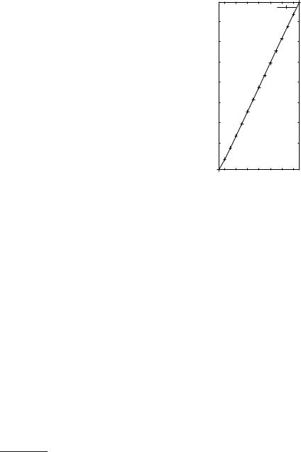
Fig. 1.1. The running time of the school method for the multiplication of n-digit integers. The three columns of the table on the left give n, the running time Tn of the C++ implementation given in Sect. 1.7, and the ratio Tn/Tn/2. The plot on the right shows log Tn versus log n, and we
see essentially a line. Observe that if Tn = α nβ for some constants α and β , then Tn/Tn/2 = 2β and log Tn = β log n + log α , i.e., log Tn depends linearly on log n with slope β . In our case, the slope is two. Please, use a ruler to check
complex transport mechanism for data between memory and the processing unit, but they will have a similar effect for all i, and hence the number of primitive operations is also representative of the running time of an actual implementation on an actual machine. The argument extends to multiplication, since multiplication of a number by a one-digit number is a process similar to addition and the second phase of the school method for multiplication amounts to a series of additions.
Let us confirm the above argument by an experiment. Figure 1.1 shows execution times of a C++ implementation of the school method; the program can be found in Sect. 1.7. For each n, we performed a large number4 of multiplications of n-digit random integers and then determined the average running time Tn; Tn is listed in the second column. We also show the ratio Tn/Tn/2. Figure 1.1 also shows a plot of the data points5 (logn, logTn). The data exhibits approximately quadratic growth, as we can deduce in various ways. The ratio Tn/Tn/2 is always close to four, and the double logarithmic plot shows essentially a line of slope two. The experiments
4The internal clock that measures CPU time returns its timings in some units, say milliseconds, and hence the rounding required introduces an error of up to one-half of this unit. It is therefore important that the experiment timed takes much longer than this unit, in order to reduce the effect of rounding.
5 Throughout this book, we use log x to denote the logarithm to base 2, log2 x.

6 1 Appetizer: Integer Arithmetics
are quite encouraging: our theoretical analysis has predictive value. Our theoretical analysis showed quadratic growth of the number of primitive operations, we argued above that the running time should be related to the number of primitive operations, and the actual running time essentially grows quadratically. However, we also see systematic deviations. For small n, the growth from one row to the next is less than by a factor of four, as linear and constant terms in the running time still play a substantial role. For larger n, the ratio is very close to four. For very large n (too large to be timed conveniently), we would probably see a factor larger than four, since the access time to memory depends on the size of the data. We shall come back to this point in Sect. 2.2.
Exercise 1.2. Write programs for the addition and multiplication of long integers. Represent integers as sequences (arrays or lists or whatever your programming language offers) of decimal digits and use the built-in arithmetic to implement the primitive operations. Then write ADD, MULTIPLY1, and MULTIPLY functions that add integers, multiply an integer by a one-digit number, and multiply integers, respectively. Use your implementation to produce your own version of Fig. 1.1. Experiment with using a larger base than base 10, say base 216.
Exercise 1.3. Describe and analyze the school method for division.
1.3 Result Checking
Our algorithms for addition and multiplication are quite simple, and hence it is fair to assume that we can implement them correctly in the programming language of our choice. However, writing software6 is an error-prone activity, and hence we should always ask ourselves whether we can check the results of a computation. For multiplication, the authors were taught the following technique in elementary school. The method is known as Neunerprobe in German, “casting out nines” in English, and preuve par neuf in French.
Add the digits of a. If the sum is a number with more than one digit, sum its digits. Repeat until you arrive at a one-digit number, called the checksum of a. We use sa to denote this checksum. Here is an example:
4528 → 19 → 10 → 1 .
Do the same for b and the result c of the computation. This gives the checksums sb and sc. All checksums are single-digit numbers. Compute sa · sb and form its checksum s. If s differs from sc, c is not equal to a · b. This test was described by al-Khwarizmi in his book on algebra.
Let us go through a simple example. Let a = 429, b = 357, and c = 154153. Then sa = 6, sb = 6, and sc = 1. Also, sa · sb = 36 and hence s = 9. So sc =s and
6The bug in the division algorithm of the floating-point unit of the original Pentium chip became infamous. It was caused by a few missing entries in a lookup table used by the algorithm.

1.4 A Recursive Version of the School Method |
7 |
hence sc is not the product of a and b. Indeed, the correct product is c = 153153. Its checksum is 9, and hence the correct product passes the test. The test is not foolproof, as c = 135153 also passes the test. However, the test is quite useful and detects many mistakes.
What is the mathematics behind this test? We shall explain a more general method. Let q be any positive integer; in the method described above, q = 9. Let sa be the remainder, or residue, in the integer division of a by q, i.e., sa = a − a/q ·q. Then 0 ≤ sa < q. In mathematical notation, sa = a mod q.7 Similarly, sb = b mod q and sc = c mod q. Finally, s = (sa · sb) mod q. If c = a · b, then it must be the case that s = sc. Thus s =sc proves c =a ·b and uncovers a mistake in the multiplication. What do we know if s = sc? We know that q divides the difference of c and a · b. If this difference is nonzero, the mistake will be detected by any q which does not divide the difference.
Let us continue with our example and take q = 7. Then a mod 7 = 2, b mod 7 = 0 and hence s = (2 · 0) mod 7 = 0. But 135153 mod 7 = 4, and we have uncovered that 135153 =429 · 357.
Exercise 1.4. Explain why the method learned by the authors in school corresponds to the case q = 9. Hint: 10k mod 9 = 1 for all k ≥ 0.
Exercise 1.5 (Elferprobe, casting out elevens). Powers of ten have very simple remainders modulo 11, namely 10k mod 11 = (−1)k for all k ≥ 0, i.e., 1 mod 11 = 1, 10 mod 11 = −1, 100 mod 11 = +1, 1 000 mod 11 = −1, etc. Describe a simple test to check the correctness of a multiplication modulo 11.
1.4 A Recursive Version of the School Method
We shall now derive a recursive version of the school method. This will be our first encounter with the divide-and-conquer paradigm, one of the fundamental paradigms in algorithm design.
Let a and b be our two n-digit integers which we want to multiply. Let k = n/2 . We split a into two numbers a1 and a0; a0 consists of the k least significant digits and a1 consists of the n − k most significant digits.8 We split b analogously. Then
a = a1 · Bk + a0 and b = b1 · Bk + b0 ,
and hence
a · b = a1 · b1 · B2k + (a1 · b0 + a0 · b1) · Bk + a0 · b0 .
This formula suggests the following algorithm for computing a · b:
7The method taught in school uses residues in the range 1 to 9 instead of 0 to 8 according to the definition sa = a − ( a/q − 1) · q.
8Observe that we have changed notation; a0 and a1 now denote the two parts of a and are no longer single digits.
81 Appetizer: Integer Arithmetics
(a)Split a and b into a1, a0, b1, and b0.
(b)Compute the four products a1 · b1, a1 · b0, a0 · b1, and a0 · b0.
(c)Add the suitably aligned products to obtain a · b.
Observe that the numbers a1, a0, b1, and b0 are n/2 -digit numbers and hence the multiplications in step (b) are simpler than the original multiplication if n/2 < n, i.e., n > 1. The complete algorithm is now as follows. To multiply one-digit numbers, use the multiplication primitive. To multiply n-digit numbers for n ≥ 2, use the threestep approach above.
It is clear why this approach is called divide-and-conquer. We reduce the problem of multiplying a and b to some number of simpler problems of the same kind. A divide-and-conquer algorithm always consists of three parts: in the first part, we split the original problem into simpler problems of the same kind (our step (a)); in the second part we solve the simpler problems using the same method (our step (b)); and, in the third part, we obtain the solution to the original problem from the solutions to the subproblems (our step (c)).
|
|
|
|
a1 |
|
|
a0 |
|
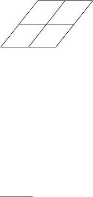
Fig. 1.2. Visualization of the school method and |
||
|
|
|
|
|
|
|
|
|
|
|
its recursive variant. The rhombus-shaped area |
|
|
|
|
a1.b0 |
|
|
a0 . b0 |
b0 |
indicates the partial products in the multiplication |
||
|
|
|
|
|
|
a · b. The four subareas correspond to the partial |
|||||
|
|
|
|
|
|
|
|
|
|
|
|
|
|
|
|
|
|
|
|
|
|
|
products a1 · b1, a1 · b0, a0 · b1, and a0 · b0. In the |
a |
|
.b |
|
a |
|
. b |
|
b |
|
|
recursive scheme, we first sum the partial prod- |
1 |
1 |
0 |
1 |
1 |
|
ucts in the four subareas and then, in a second |
|||||
|
|
|
|
|
|
||||||
step, add the four resulting sums
What is the connection of our recursive integer multiplication to the school method? It is really the same method. Figure 1.2 shows that the products a1 · b1, a1 · b0, a0 · b1, and a0 · b0 are also computed in the school method. Knowing that our recursive integer multiplication is just the school method in disguise tells us that the recursive algorithm uses a quadratic number of primitive operations. Let us also derive this from first principles. This will allow us to introduce recurrence relations, a powerful concept for the analysis of recursive algorithms.
Lemma 1.4. Let T (n) be the maximal number of primitive operations required by our recursive multiplication algorithm when applied to n-digit integers. Then
T (n) ≤ |
4 |
|
T ( n/2 ) + 3 2 n if n |
= 2. |
|
|
1 |
|
|
if n |
1, |
|
|
· |
· · |
|
≥ |
Proof. Multiplying two one-digit numbers requires one primitive multiplication. This justifies the case n = 1. So, assume n ≥ 2. Splitting a and b into the four pieces a1, a0, b1, and b0 requires no primitive operations.9 Each piece has at most n/2
9 It will require work, but it is work that we do not account for in our analysis.

1.5 Karatsuba Multiplication |
9 |
digits and hence the four recursive multiplications require at most 4 ·T ( n/2 ) primitive operations. Finally, we need three additions to assemble the final result. Each addition involves two numbers of at most 2n digits and hence requires at most 2n primitive operations. This justifies the inequality for n ≥ 2.
In Sect. 2.6, we shall learn that such recurrences are easy to solve and yield the already conjectured quadratic execution time of the recursive algorithm.
Lemma 1.5. Let T (n) be the maximal number of primitive operations required by our recursive multiplication algorithm when applied to n-digit integers. Then T (n) ≤ 7n2 if n is a power of two, and T (n) ≤ 28n2 for all n.
Proof. We refer the reader to Sect. 1.8 for a proof. |
|
1.5 Karatsuba Multiplication
In 1962, the Soviet mathematician Karatsuba [104] discovered a faster way of multiplying large integers. The running time of his algorithm grows like nlog3 ≈ n1.58. The method is surprisingly simple. Karatsuba observed that a simple algebraic identity allows one multiplication to be eliminated in the divide-and-conquer implementation, i.e., one can multiply n-bit numbers using only three multiplications of integers half the size.
The details are as follows. Let a and b be our two n-digit integers which we want to multiply. Let k = n/2 . As above, we split a into two numbers a1 and a0; a0 consists of the k least significant digits and a1 consists of the n − k most significant digits. We split b in the same way. Then
a = a1 · Bk + a0 and b = b1 · Bk + b0
and hence (the magic is in the second equality)
a · b = a1 · b1 · B2k + (a1 · b0 + a0 · b1) · Bk + a0 · b0
= a1 · b1 · B2k + ((a1 + a0) · (b1 + b0) − (a1 · b1 + a0 · b0)) · Bk + a0 · b0 .
At first sight, we have only made things more complicated. A second look, how-
ever, shows that the last formula can be evaluated with only three multiplications, namely, a1 · b1, a1 · b0, and (a1 + a0) · (b1 + b0). We also need six additions.10 That
is three more than in the recursive implementation of the school method. The key is that additions are cheap compared with multiplications, and hence saving a multiplication more than outweighs three additional additions. We obtain the following algorithm for computing a · b:
10Actually, five additions and one subtraction. We leave it to readers to convince themselves that subtractions are no harder than additions.