

Algorithms and data structures
.pdf9.2 Depth-First Search |
183 |
cycles. In this case, all SCCs lying on one of the newly formed cycles are merged into a single SCC, and the shrunken graph changes accordingly.
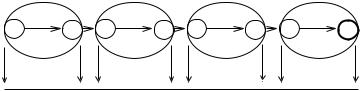
In order to arrive at an efficient algorithm, we need to describe how we maintain the SCCs as the graph evolves. If the edges are added in arbitrary order, no efficient simple method is known. However, if we use DFS to explore the graph, an efficient solution is fairly simple to obtain. Consider a depth-first search on G and let Ec be the set of edges already explored by DFS. A subset Vc of the nodes is already marked. We distinguish between three kinds of SCC of Gc: unreached, open, and closed. Unmarked nodes have indegree and outdegree zero in Gc and hence form SCCs consisting of a single node. This node is isolated in the shrunken graph. We call these SCCs unreached. The other SCCs consist of marked nodes only. We call an SCC consisting of marked nodes open if it contains an active node, and closed if it contains only finished nodes. We call a marked node “open” if it belongs to an open component and “closed” if it belongs to a closed component. Observe that a closed node is always finished and that an open node may be either active or finished. For every SCC, we call the node with the smallest DFS number in the SCC the representative of the SCC. Figure 9.6 illustrates these concepts. We state next some important invariant properties of Gc; see also Fig. 9.7:
(1)All edges in G (not just Gc) out of closed nodes lead to closed nodes. In our example, the nodes a and e are closed.
(2)The tree path to the current node contains the representatives of all open components. Let S1 to Sk be the open components as they are traversed by the tree path to the current node. There is then a tree edge from a node in Si−1 to the representative of Si, and this is the only edge into Si, 2 ≤ i ≤ k. Also, there is no
edge from an S j to an Si with i < j. Finally, all nodes in S j are reachable from the representative ri of Si for 1 ≤ i ≤ j ≤ k. In short, the open components form a path in the shrunken graph. In our example, the current node is g. The tree pathb, c, f , g to the current node contains the open representatives b, c, and f .
(3)Consider the nodes in open components ordered by their DFS numbers. The representatives partition the sequence into the open components. In our example, the sequence of open nodes is b, c, d, f , g, h and the representatives partition this sequence into the open components {b}, {c, d}, and { f , g, h}.
We shall show below that all three properties hold true generally, and not only for our example. The three properties will be invariants of the algorithm to be developed. The first invariant implies that the closed SCCs of Gc are actually SCCs of G, i.e., it is justified to call them closed. This observation is so important that it deserves to be stated as a lemma.
Lemma 9.5. A closed SCC of Gc is an SCC of G.
Proof. Let v be a closed vertex, let S be the SCC of G containing v, and let Sc be the SCC of Gc containing v. We need to show that S = Sc. Since Gc is a subgraph of G, we have Sc S. So, it suffices to show that S Sc. Let w be any vertex in S. There is then a cycle C in G passing through v and w. The first invariant implies that
184 9 Graph Traversal
all vertices of C are closed. Since closed vertices are finished, all edges out of them have been explored. Thus C is contained in Gc, and hence w Sc.
The Invariants (2) and (3) suggest a simple method to represent the open SCCs of Gc. We simply keep a sequence oNodes of all open nodes in increasing order of DFS numbers, and the subsequence oReps of open representatives. In our example, we have oNodes = b, c, d, f , g, h and oReps = b, c, f . We shall later see that the type Stack of NodeId is appropriate for both sequences.
Let us next see how the SCCs of Gc develop during DFS. We shall discuss the various actions of DFS one by one and show that the invariants are maintained. We shall also discuss how to update our representation of the open components.
When DFS starts, the invariants clearly hold: no node is marked, no edge has been traversed, Gc is empty, and hence there are neither open nor closed components yet. Our sequences oNodes and oReps are empty.
Just before a new root will be marked, all marked nodes are finished and hence there cannot be any open component. Therefore, both of the sequences oNodes and oReps are empty, and marking a new root s produces the open component {s}. The invariants are clearly maintained. We obtain the correct representation by adding s to both sequences.
If a tree edge e = (v, w) is traversed and hence w becomes marked, {w} becomes an open component on its own. All other open components are unchanged. The first invariant is clearly maintained, since v is active and hence open. The old current node is v and the new current node is w. The sequence of open components is extended by {w}. The open representatives are the old open representatives plus the node w. Thus the second invariant is maintained. Also, w becomes the open node with the largest DFS number and hence oNodes and oReps are both extended by w. Thus the third invariant is maintained.
Now suppose that a nontree edge e = (v, w) out of the current node v is explored. If w is closed, the SCCs of Gc do not change when e is added to Gc since, by Lemma 9.5, the SCC of Gc containing w is already an SCC of G before e is traversed. So, assume that w is open. Then w lies in some open SCC Si of Gc. We claim
S1 |
S2 |
|
Sk |
|
r1 |
r2 |
rk |
current |
|
node |
||||
|
|
|
open nodes ordered by dfsNum
Fig. 9.7. The open SCCs are shown as ovals, and the current node is shown as a bold circle. The tree path to the current node is indicated. It enters each component at its representative. The horizontal line below represents the open nodes, ordered by dfsNum. Each open SCC forms a contiguous subsequence, with its representative as its leftmost element

9.2 |
Depth-First Search |
185 |
||
Si |
|
Sk |
|
|
ri |
rk |
v |
current |
|
node |
|
|||
|
|
|
|
|
w
Fig. 9.8. The open SCCs are shown as ovals and their representatives as circles to the left of an oval. All representatives lie on the tree path to the current node v. The nontree edge e = (v, w) ends in an open SCC Si with representative ri. There is a path from w to ri since w belongs to the SCC with representative ri. Thus the edge (v, w) merges Si to Sk into a single SCC
that the SCCs Si to Sk are merged into a single component and all other components are unchanged; see Fig. 9.8. Let ri be the representative of Si. We can then go from ri to v along a tree path by invariant (2), then follow the edge (v, w), and finally return to ri. The path from w to ri exists, since w and ri lie in the same SCC of Gc. We conclude that any node in an S j with i ≤ j ≤ k can be reached from ri and can reach ri. Thus the SCCs Si to Sk become one SCC, and ri is their representative. The S j with j < i are unaffected by the addition of the edge.
The third invariant tells us how to find ri, the representative of the component containing w. The sequence oNodes is ordered by dfsNum, and the representative of an SCC has the smallest dfsNum of any node in that component. Thus dfsNum[ri] ≤ dfsNum[w] and dfsNum[w] < dfsNum[r j] for all j > i. It is therefore easy to update our representation. We simply delete all representatives r with dfsNum[r] > dfsNum[w] from oReps.
Finally, we need to consider finishing a node v. When will this close an SCC? By invariant (2), all nodes in a component are tree descendants of the representative of the component, and hence the representative of a component is the last node to be finished in the component. In other words, we close a component iff we finish a representative. Since oReps is ordered by dfsNum, we close a component iff the last node of oReps finishes. So, assume that we finish a representative v. Then, by invariant (3), the component Sk with representative v = rk consists of v and all nodes in oNodes following v. Finishing v closes Sk. By invariant (2), there is no edge out of Sk into an open component. Thus invariant (1) holds after Sk is closed. The new current node is the parent of v. By invariant (2), the parent of v lies in Sk−1. Thus invariant (2) holds after Sk is closed. Invariant (3) holds after v is removed from oReps, and v and all nodes following it are removed from oNodes.
It is now easy to instantiate the DFS template. Fig. 9.10 shows the pseudocode, and Fig. 9.9 illustrates a complete run. We use an array component indexed by nodes to record the result, and two stacks oReps and oNodes. When a new root is marked or a tree edge is explored, a new open component consisting of a single node is created by pushing this node onto both stacks. When a cycle of open components is created, these components are merged by popping representatives from oReps as long as the top representative is not to the left of the node w closing the cycle. An SCC S is closed when its representative v finishes. At that point, all nodes of S are stored
186 |
9 Graph Traversal |
|
|
|
|
||
a b c d e |
f g h i j k |
a b c d e f g h i j k |
|||||
|
|
|
|
traverse(e,g) |
traverse(e,h) |
traverse(h,i) |
|
root(a) |
traverse(a,b) traverse(b,c) |
traverse(i,e) |
|
|
|||
|
|
|
|
|
|
||
traverse(c,a) |
|
|
traverse(i,j) traverse(j,c) |
traverse(j,k) |
|||
|
|
|
|
||||
backtrack(b,c) |
backtrack(a,b) |
traverse(k,d) |
|
|
|||
|
|
|
|
|
|
||
backtrack(a,a) |
|
|
|
|
|
|
|
|
|
|
|
backtrack(j,k) |
backtrack(i,j) |
backtrack(h,i) |
|
root(d) |
traverse(d,e) traverse(e,f) traverse(f,g) |
backtrack(e,h) |
backtrack(d,e) |
|
|||
|
|
|
|
||||
backtrack(f,g) |
backtrack(e,f) |
backtrack(d,d) |
|
|
|||
|
|
|
|
|
|
||
unmarked marked |
finished |
|
nontraversed edge |
closed SCC |
|||
|
|
|
nonrepresentative node |
||||
|
|
|
representative node |
traversed edge |
open SCC |
||
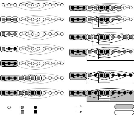
Fig. 9.9. An example of the development of open and closed SCCs during DFS. Unmarked nodes are shown as empty circles, marked nodes are shown in gray, and finished nodes are shown in black. Nontraversed edges are shown in gray, and traversed edges are shown in black. Open SCCs are shown as empty ovals, and closed SCCs are shown as gray ovals. We start in the situation shown at the upper left. We make a a root and traverse the edges (a, b) and (b, c). This creates three open SSCs. The traversal of edge (c, a) merges these components into one. Next, we backtrack to b, then to a, and finally from a. At this point, the component becomes closed. Please complete the description
above v in oNodes. The operation backtrack therefore closes S by popping v from oReps, and by popping the nodes w S from oNodes and setting their component to the representative v.
Note that the test w oNodes in traverseNonTreeEdge can be done in constant time by storing information with each node that indicates whether the node is open or not. This indicator is set when a node v is first marked, and reset when the component of v is closed. We give implementation details in Sect. 9.3. Furthermore, the while loop and the repeat loop can make at most n iterations during the entire execution of the algorithm, since each node is pushed onto the stacks exactly once. Hence, the execution time of the algorithm is O(m + n). We have the following theorem.
|
9.2 Depth-First Search |
187 |
init: |
|
|
component : NodeArray of NodeId |
// SCC representatives |
|
oReps = : Stack of NodeId |
// representatives of open SCCs |
|
oNodes = : Stack of NodeId |
// all nodes in open SCCs |
|
root(w) or traverseTreeEdge(v, w): |
|
|
oReps.push(w) |
// new open |
|
oNodes.push(w) |
// component |
|
traverseNonTreeEdge(v, w): |
|
|
if w oNodes then |
|
|
while w oReps.top do oReps.pop |
// collapse components on cycle |
|
backtrack(u, v): |
|
|
if v = oReps.top then |
|
|
oReps.pop |
// |
close |
repeat |
// component |
|
w := oNodes.pop |
|
|
component[w] := v until w = v
Fig. 9.10. An instantiation of the DFS template that computes strongly connected components of a graph G = (V, E)
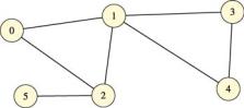
Fig. 9.11. The graph has two 2-edge connected components, namely {0, 1, 2, 3, 4} and {5}. The graph has three biconnected components, namely the subgraphs spanned by the sets {0, 1, 2}, {1, 3, 4} and {2, 5}. The vertices 1 and 2 are articulation points
Theorem 9.6. The algorithm in Fig. 9.10 computes strongly connected components in time O(m + n).
Exercise 9.14 (certificates). Let G be a strongly connected graph and let s be a node of G. Show how to construct two trees rooted at s. The first tree proves that all nodes can be reached from s, and the second tree proves than s can be reached from all nodes.
Exercise 9.15 (2-edge-connected components). An undirected graph is 2-edge- connected if its edges can be oriented so that the graph becomes strongly connected. The 2-edge-connected components are the maximal 2-edge-connected subgraphs; see Fig. 9.11. Modify the SCC algorithm shown in Fig. 9.10 so that it computes 2- edge-connected components. Hint: show first that DFS of an undirected graph never produces any cross edges.
188 9 Graph Traversal
Exercise 9.16 (biconnected components). Two nodes of an undirected graph belong to the same biconnected component (BCC) iff they are connected by an edge or there are two edge-disjoint paths connecting them; see Fig. 9.11. A node is an articulation point if it belongs to more than one BCC. Design an algorithm that computes biconnected components using a single pass of DFS. Hint: adapt the strongly- connected-components algorithm. Define the representative of a BCC as the node with the second smallest dfsNum in the BCC. Prove that a BCC consists of the parent of the representative and all tree descendants of the representative that can be reached without passing through another representative. Modify backtrack. When you return from a representative v, output v, all nodes above v in oNodes, and the parent of v.
9.3 Implementation Notes
BFS is usually implemented by keeping unexplored nodes (with depths d and d + 1) in a FIFO queue. We chose a formulation using two separate sets for nodes at depth d and nodes at depth d + 1 mainly because it allows a simple loop invariant that makes correctness immediately evident. However, our formulation might also turn out to be somewhat more efficient. If Q and Q are organized as stacks, we will have fewer cache faults than with a queue, in particular if the nodes of a layer do not quite fit into the cache. Memory management becomes very simple and efficient when just a single array a of n nodes is allocated for both of the stacks Q and Q . One stack grows from a[1] to the right and the other grows from a[n] to the left. When the algorithm switches to the next layer, the two memory areas switch their roles.
Our SCC algorithm needs to store four kinds of information for each node v: an indication of whether v is marked, an indication of whether v is open, something like a DFS number in order to implement “ ”, and, for closed nodes, the NodeId of the representative of its component. The array component suffices to keep this information. For example, if NodeIds are integers in 1..n, component[v] = 0 could indicate an unmarked node. Negative numbers can indicate negated DFS numbers, so that u v iff component[u] > component[v]. This works because “ ” is never applied to closed nodes. Finally, the test w oNodes simply becomes component[v] < 0. With these simplifications in place, additional tuning is possible. We make oReps store component numbers of representatives rather than their IDs, and save an access to component[oReps.top]. Finally, the array component should be stored with the node data as a single array of records. The effect of these optimization on the performance of our SCC algorithm is discussed in [132].
9.3.1 C++
LEDA [118] has implementations for topological sorting, reachability from a node (DFS), DFS numbering, BFS, strongly connected components, biconnected components, and transitive closure. BFS, DFS, topological sorting, and strongly connected
9.4 Historical Notes and Further Findings |
189 |
components are also available in a very flexible implementation that separates representation and implementation, supports incremental execution, and allows various other adaptations.
The Boost graph library [27] uses the visitor concept to support graph traversal. A visitor class has user-definable methods that are called at event points during the execution of a graph traversal algorithm. For example, the DFS visitor defines event points similar to the operations init, root, traverse , and backtrack used in our DFS template; there are more event points in Boost.
9.3.2 Java
The JDSL [78] library [78] supports DFS in a very flexible way, not very much different from the visitor concept described for Boost. There are also more specialized algorithms for topological sorting and finding cycles.
9.4 Historical Notes and Further Findings
BFS and DFS were known before the age of computers. Tarjan [185] discovered the power of DFS and provided linear-time algorithms for many basic problems related to graphs, in particular biconnected and strongly connected components. Our SCC algorithm was invented by Cheriyan and Mehlhorn [39] and later rediscovered by Gabow [70]. Yet another linear-time SCC algorithm is that due to Kosaraju and Sharir [178]. It is very simple, but needs two passes of DFS. DFS can be used to solve many other graph problems in linear time, for example ear decomposition, planarity testing, planar embeddings, and triconnected components.
It may seem that problems solvable by graph traversal are so simple that little further research is needed on them. However, the bad news is that graph traversal itself is very difficult on advanced models of computation. In particular, DFS is a nightmare for both parallel processing [161] and memory hierarchies [141, 128]. Therefore alternative ways to solve seemingly simple problems are an interesting area of research. For example, in Sect. 11.8 we describe an approach to constructing minimum spanning trees using edge contraction that also works for finding connected components. Furthermore, the problem of finding biconnected components can be reduced to finding connected components [189]. The DFS-based algorithms for biconnected components and strongly connected components are almost identical. But this analogy completely disappears for advanced models of computation, so that algorithms for strongly connected components remain an area of intensive (and sometimes frustrating) research. More generally, it seems that problems for undirected graphs (such as finding biconnected components) are often easier to solve than analogous problems for directed graphs (such as finding strongly connected components).
10
Shortest Paths
M |
0 |
Distance to M
 R 5
R 5
|
|
|
L |
|
11 |
|
|
|
O |
|
13 |
|
|
|
Q |
|
15 |
|
G N |
S |
17 |
18 17 |
|
|
F |
K |
P |
19 |
20 |
|
|
|
|
||
H |
|
E |
J |
|
|
|
|
|
|
||
C V
W
The problem of the shortest, quickest or cheapest path is ubiquitous. You solve it daily. When you are in a location s and want to move to a location t, you ask for the quickest path from s to t. The fire department may want to compute the quickest routes from a fire station s to all locations in town – the single-source problem. Sometimes we may even want a complete distance table from everywhere to everywhere – the all-pairs problem. In a road atlas, you will usually find an all-pairs distance table for the most important cities.
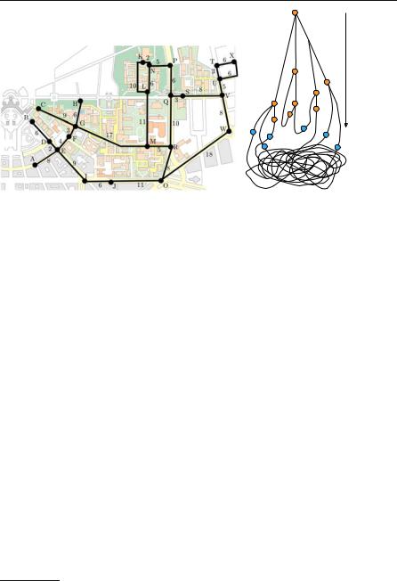
Here is a route-planning algorithm that requires a city map and a lot of dexterity but no computer. Lay thin threads along the roads on the city map. Make a knot wherever roads meet, and at your starting position. Now lift the starting knot until the entire net dangles below it. If you have successfully avoided any tangles and the threads and your knots are thin enough so that only tight threads hinder a knot from moving down, the tight threads define the shortest paths. The introductory figure of this chapter shows the campus map of the University of Karlsruhe1 and illustrates the route-planning algorithm for the source node M.
Route planning in road networks is one of the many applications of shortestpath computations. When an appropriate graph model is deÞned, many problems turn out to proÞt from shortest-path computations. For example, Ahuja et al. [8] mentioned such diverse applications as planning ßows in networks, urban housing, inventory planning, DNA sequencing, the knapsack problem (see also Chap. 12), production planning, telephone operator scheduling, vehicle ßeet planning, approximating piecewise linear functions, and allocating inspection effort on a production line.
The most general formulation of the shortest-path problem looks at a directed graph G = (V, E) and a cost function c that maps edges to arbitrary real-number
1 (c) UniversitŠt Karlsruhe (TH), Institut fŸr Photogrammetrie und Fernerkundung.

192 10 Shortest Paths
costs. It turns out that the most general problem is fairly expensive to solve. So we are also interested in various restrictions that allow simpler and more efÞcient algorithms: nonnegative edge costs, integer edge costs, and acyclic graphs. Note that we have already solved the very special case of unit edge costs in Sect. 9.1 Ð the breadth-Þrst search (BFS) tree rooted at node s is a concise representation of all shortest paths from s. We begin in Sect. 10.1 with some basic concepts that lead to a generic approach to shortest-path algorithms. A systematic approach will help us to keep track of the zoo of shortest-path algorithms. As our Þrst example of a restricted but fast and simple algorithm, we look at acyclic graphs in Sect. 10.2. In Sect. 10.3, we come to the most widely used algorithm for shortest paths: DijkstraÕs algorithm for general graphs with nonnegative edge costs. The efÞciency of DijkstraÕs algorithm relies heavily on efÞcient priority queues. In an introductory course or at Þrst reading, DijkstraÕs algorithm might be a good place to stop. But there are many more interesting things about shortest paths in the remainder of the chapter. We begin with an average-case analysis of DijkstraÕs algorithm in Sect. 10.4 which indicates that priority queue operations might dominate the execution time less than one might think. In Sect. 10.5, we discuss monotone priority queues for integer keys that take additional advantage of the properties of DijkstraÕs algorithm. Combining this with average-case analysis leads even to a linear expected execution time. Section 10.6 deals with arbitrary edge costs, and Sect. 10.7 treats the all-pairs problem. We show that the all-pairs problem for general edge costs reduces to one general single-source problem plus n single-source problems with nonnegative edge costs. This reduction introduces the generally useful concept of node potentials. We close with a discussion of shortest path queries in Sect. 10.8.
10.1 From Basic Concepts to a Generic Algorithm
We extend the cost function to paths in the natural way. The cost of a path is the sum of the costs of its constituent edges, i.e., if p = e1, e2, . . . , ek , then c(p) = ∑1≤i≤k c(ei). The empty path has cost zero.
For a pair s and v of nodes, we are interested in a shortest path from s to v. We avoid the use of the deÞnite article ÒtheÓ here, since there may be more than one shortest path. Does a shortest path always exist? Observe that the number of paths from s to v may be inÞnite. For example, if r = pCq is a path from s to v containing a cycle C, then we may go around the cycle an arbitrary number of times and still have a path from s to v; see Fig. 10.1. More precisely, p is a path leading from s to u, C is a path leading from u to u, and q is a path from u to v. Consider the path r(i) = pCiq which Þrst uses p to go from s to u, then goes around the cycle i times, and Þnally follows q from u to v. The cost of r(i) is c(p) + i ·c(C) + c(q). If C is a negative cycle, i.e., c(C) < 0, then c(r(i+1)) < c(r(i)). In this situation, there is no shortest path from s to v. Assume otherwise: say, P is a shortest path from s to v. Then c(r(i)) < c(P) for i large enough2, and so P is not a shortest path from s to v. We shall show next that shortest paths exist if there are no negative cycles.
2 i > (c( p) + c(q) − c(P))/|c(C)| will do.
|
|
10.1 |
From Basic Concepts to a Generic Algorithm |
193 |
||||
s p |
|
q |
v s p |
|
C |
(2) q |
v ... |
|
|
u |
C |
|
u |
|
|
|
|
|
|
|
|
|
|
|
||
Fig. 10.1. A nonsimple path pCq from s to v
Lemma 10.1. If G contains no negative cycles and v is reachable from s, then a shortest path P from s to v exists. Moreover P can be chosen to be simple.
Proof. Let x be a shortest simple path from s to v. If x is not a shortest path from s to v, there is a shorter nonsimple path r from s to v. Since r is nonsimple we can, as in Fig. 10.1, write r as pCq, where C is a cycle and pq is a simple path. Then c(x) ≤ c( pq), and hence c( pq) + c(C) = c(r) < c(x) ≤ c(pq). So c(C) < 0 and we have shown the existence of a negative cycle.
Exercise 10.1. Strengthen the lemma above and show that if v is reachable from s, then a shortest path from s to v exists iff there is no negative cycle that is reachable from s and from which one can reach v.
For two nodes s and v, we deÞne the shortest-path distance μ (s, v) from s to v as
|
+∞ |
if there is no path from s to v, |
|
μ (s, v) := |
− |
∞ |
if there is no shortest path from s to v, |
|
|||
|
c (a shortest path from s to v) |
otherwise. |
|
Since we use s to denote the source vertex most of the time, we also use the shorthand μ (v) := μ (s, v). Observe that if v is reachable from s but there is no shortest path from s to v, then there are paths of arbitrarily large negative cost. Thus it makes sense to deÞne μ (v) = −∞ in this case. Shortest paths have further nice properties, which we state as exercises.
Exercise 10.2 (subpaths of shortest paths). Show that subpaths of shortest paths are themselves shortest paths, i.e., if a path of the form pqr is a shortest path, then q is also a shortest path.
Exercise 10.3 (shortest-path trees). Assume that all nodes are reachable from s and that there are no negative cycles. Show that there is an n-node tree T rooted at s such that all tree paths are shortest paths. Hint: assume Þrst that shortest paths are unique, and consider the subgraph T consisting of all shortest paths starting at s. Use the preceding exercise to prove that T is a tree. Extend this result to the case where shortest paths are not unique.
Our strategy for Þnding shortest paths from a source node s is a generalization of the BFS algorithm shown in Fig. 9.3. We maintain two NodeArrays d and parent. Here, d[v] contains our current knowledge about the distance from s to v, and parent[v] stores the predecessor of v on the current shortest path to v. We usually