

Algorithms and data structures
.pdf60 3 Representing Sequences by Arrays and Linked Lists
bounded arrays, which can grow and shrink as elements are inserted and removed. The analysis of unbounded arrays introduces the concept of amortized analysis.
The second way of referring to the elements of a sequence is relative to other elements. For example, one could ask for the successor of an element e, the predecessor of an element e , or for the subsequence e, . . . , e of elements between e and e . Although relative access can be simulated using array indexing, we shall see in Sect. 3.1 that a list-based representation of sequences is more flexible. In particular, it becomes easier to insert or remove arbitrary pieces of a sequence.
Many algorithms use sequences in a quite limited way. Only the front and/or the rear of the sequence are read and modified. Sequences that are used in this restricted way are called stacks, queues, and deques. We discuss them in Sect. 3.4. In Sect. 3.5, we summarize the findings of the chapter.
3.1 Linked Lists
In this section, we study the representation of sequences by linked lists. In a doubly linked list, each item points to its successor and to its predecessor. In a singly linked list, each item points to its successor. We shall see that linked lists are easily modified in many ways: we may insert or delete items or sublists, and we may concatenate lists. The drawback is that random access (the operator [·]) is not supported. We study doubly linked lists in Sect. 3.1.1, and singly linked lists in Sect. 3.1.2. Singly linked lists are more space-efficient, and somewhat faster, and should therefore be preferred whenever their functionality suffices. A good way to think of a linked list is to imagine a chain, where one element is written on each link. Once we get hold of one link of the chain, we can retrieve all elements.
3.1.1 Doubly Linked Lists
Figure 3.1 shows the basic building blocks of a linked list. A list item stores an element, and pointers to its successor and predecessor. We call a pointer to a list item a handle. This sounds simple enough, but pointers are so powerful that we can make a big mess if we are not careful. What makes a consistent list data structure? We
Class Handle = Pointer to Item |
|
|
|
|
|
|
|
|
|
|
|
|
|
Class Item of Element |
|
|
// one link in a doubly linked list |
|
|||||||||
e : Element |
// |
|
|
|
|
|
|
|
|
|
|
||
|
|
|
|
|
|
|
|||||||
next : Handle |
|
|
|
|
|
|
|
||||||
|
|
|
|
|
|
|
|
|
|
|
|||
|
|
|
|
|
|||||||||
prev : Handle |
|
|
|
|
|
|
|
|
|
|
|
|
|
|
|
|
|
|
|
|
|
|
|
|
|
|
|
invariant next→prev = prev→next = this |
|
|
|
|
|
|
|
|
|
|
|
|
|
Fig. 3.1. The items of a doubly linked list
3.1 Linked Lists |
61 |
|
e1 |
|
|
en |
|
|
|
··· |
|
|
|
··· |
|
|
|
|
|
|
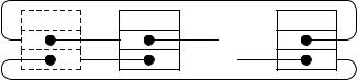
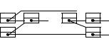
Fig. 3.2. The representation of a sequence e1, . . . , en by a doubly linked list. There are n + 1 items arranged in a ring, a special dummy item h containing no element, and one item for each element of the sequence. The item containing ei is the successor of the item containing ei−1 and the predecessor of the item containing ei+1. The dummy item is between the item containing en and the item containing e1
require that for each item it, the successor of its predecessor is equal to it and the predecessor of its successor is also equal to it.
A sequence of n elements is represented by a ring of n+ 1 items. There is a special dummy item h, which stores no element. The successor h1 of h stores the first element of the sequence, the successor of h1 stores the second element of the sequence, and so on. The predecessor of h stores the last element of the sequence; see Fig. 3.2. The empty sequence is represented by a ring consisting only of h. Since there are no elements in that sequence, h is its own successor and predecessor. Figure 3.4 defines a representation of sequences by lists. An object of class List contains a single list item h. The constructor of the class initializes the header h to an item containing and having itself as successor and predecessor. In this way, the list is initialized to the empty sequence.
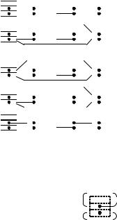
We implement all basic list operations in terms of the single operation splice shown in Fig. 3.3. splice cuts out a sublist from one list and inserts it after some target item. The sublist is specified by handles a and b to its first and its last element, respectively. In other words, b must be reachable from a by following zero or more next pointers but without going through the dummy item. The target item t can be either in the same list or in a different list; in the former case, it must not be inside the sublist starting at a and ending at b.
splice does not change the number of items in the system. We assume that there is one special list, freeList, that keeps a supply of unused elements. When inserting new elements into a list, we take the necessary items from freeList, and when removing elements, we return the corresponding items to freeList. The function checkFreeList allocates memory for new items when necessary. We defer its implementation to Exercise 3.3 and a short discussion in Sect. 3.6.
With these conventions in place, a large number of useful operations can be implemented as one-line functions that all run in constant-time. Thanks to the power of splice, we can even manipulate arbitrarily long sublists in constant-time. Figures 3.4 and 3.5 show many examples. In order to test whether a list is empty, we simply check whether h is its own successor. If a sequence is nonempty, its first and its last element are the successor and predecessor, respectively, of h. In order to move an item b to the positions after an item a , we simply cut out the sublist starting and ending at b and insert it after a . This is exactly what splice(b, b, a ) does. We move
62 3 Representing Sequences by Arrays and Linked Lists
//Remove a, . . . , b from its current list and insert it after t
//. . . , a , a, . . . , b, b , . . . + . . . , t, t , . . . → . . . , a , b , . . . + . . . , t, a, . . . , b, t , . . .
Procedure splice(a,b,t : Handle)
assert a and b belong to the same list, b is not before a, and t a, . . . , b
// |
cut out a, . . . , b |
|
|
|
a |
|
a |
|
|
|
b |
|
|
b |
|
|
|||||||||
a := a |
prev |
|
|
|
|
|
|
|
|
|
|
··· |
|
|
|
|
|
|
|
|
|
|
|||
b |
|
: b |
→ next |
|
|
|
|
|
|
|
|
··· |
|
|
|
|
|
|
|
|
|
|
|
||
|
|
= |
→ |
|
|
|
|
|
|
|
|
|
|
|
|
|
|
|
|
|
|
|
|
|
|
a |
next := b |
// |
|
|
|
|
|
|
|
|
|
|
|
|
|
|
|
|
|
|
|
||||
|
|
|
|
|
|
|
|
|
|
|
|
|
|
|
|
|
|
|
|||||||
b |
→ prev := a |
// |
|
|
|
|
|
|
|
|
··· |
|
|
|
|
|
|
|
|
||||||
|
|
|
|
··· |
|
|
|
|
|
|
|
|
|
|
|
||||||||||
|
|
→ |
|
|
|
|
|
|
|
|
|
|
|
|
|
|
|
|
|
|
|
|
|
||
|
|
|
|
|
|
|
|
|
|
|
|
|
|
|
|
|
|
|
|
||||||
// |
|
|
|
|
t |
a |
|
b |
|
|
t |
|
|
|
|
||||||||||
insert a, . . . , b after t |
|
|
|
|
|
|
|
|
|
|
|
|
|||||||||||||
|
|
|
|
|
|
|
|
|
|
··· |
|
|
|
|
|
|
|
||||||||
|
|
|
|
|
|
|
|
|
|
|
|
|
|
||||||||||||
t := t → next |
// |
|
|
|
|
|
|
|
|
|
|
|
|
|
|
|
|
|
|
|
|||||
|
|
|
|
··· |
|
|
|
|
|
|
|
|
|
|
|||||||||||
|
|
|
|
|
|
|
|
|
|
|
|
|
|||||||||||||
|
|
|
|
|
|
|
|
|
|
|
|
||||||||||||||
|
|
|
|
|
|
|
|
|
|
|
|
|
|
|
|||||||||||
b |
|
next := t |
// |
|
|
|
|
|
|
|
|
|
|
|
|
|
|
|
|
|
|
|
|||
|
|
|
|
|
|
|
|
|
|
|
|
|
|
|
|
|
|
|
|
||||||
a |
→ prev := t |
// |
|
|
|
|
|
|
|
|
··· |
|
|
|
|
|
|
|
|
||||||
|
|
|
|
··· |
|
|
|
|
|
|
|
|
|
|
|
||||||||||
|
→ |
|
|
|
|
|
|
|
|
|
|
|
|
|
|
|
|
|
|
|
|
|
|||
|
|
|
|
|
|
|
|
|
|
|
|
|
|
|
|
|
|
|
|||||||
|
|
|
|
|
|
|
|
|
|
|
|
|
|
|
|
|
|
|
|
|
|||||
t → next := a |
// |
|
|
|
|
|
|
|
|
|
··· |
|
|
|
|
|
|
|
|
||||||
|
|
|
|
|
|
|
|
|
|
|
|
|
|||||||||||||
t → prev := b |
// |
|
|
|
|
|
|
|
|
|
|
|
|
|
|
|
|
|
|
|
|||||
|
|
|
|
··· |
|
|
|
|
|
|
|
|
|
||||||||||||
|
|
|
|
|
|
|
|
|
|
|
|
|
|
||||||||||||
|
|
|
|
|
|
|
|
|
|
|
|
|
|
|
|
||||||||||
|
|
|
Fig. 3.3. Splicing lists |
|
|
|
|
|
|
|
|
|
|
|
|
|
|
|
|
|
|||||
Class List of Element |
|
|
|
|
|
|
|
|
|
|
|
|
|
|
|
|
|
|
|
|
|
|
|||
// |
Item h is the predecessor of the first element and the successor of the last element. |
|
|
|
|
||||||||||||||||||||
|
|
|
|
|
|
|
|
|
|
|
|
|
|
|
|
|
|
|
|
|
|
|
|
|
|
h = this : Item |
|
|
|
|
|
|
|
|
|
|
|
|
|
|
|
|
|
|
|
|
|||||
|
|
|
|
|
|
|
|
|
|
|
|
|
|
|
|
|
|
||||||||
|
|
|
|
|
|
|
|
|
|
|
|
|
|
|
|
|
|||||||||
|
|
// init to empty sequence |
|
|
|
|
|||||||||||||||||||
// |
this |
|
|
|
|
|
|
|
|
|
|
|
|
|
|
|
|
|
|
|
|
|
|
||
|
|
|
|
|
|
|
|
|
|
|
|
|
|
|
|
|
|
|
|
|
|
||||
Simple access functions |
|
|
|
|
|
|
|
|
|
|
|
|
|
|
|
|
|
|
|
|
|
|
|||
Function head() : Handle; return address of h |
|
|
|
// Pos. before any proper element |
|||||||||||||||||||||
Function isEmpty : {0, 1}; return h.next = this |
|
|
|
|
|
|
|
|
|
|
|
|
|
|
|
|
// ? |
|
|||||||
Function first : Handle; assert ¬isEmpty; return h.next |
|
|
|
|
|
|
|
|
|
|
|
|
|
|
|
|
|
||||||||
Function last : Handle; assert ¬isEmpty; return h.prev |
|
|
|
|
|
|
|
|
|
|
|
|
|
|
|
|
|
||||||||
//Moving elements around within a sequence.
//( . . . , a, b, c . . . , a , c , . . . ) → ( . . . , a, c . . . , a , b, c , . . . )
Procedure moveAfter(b, a : Handle) splice(b, b, a )
Procedure moveToFront(b : Handle) moveAfter(b, head)
Procedure moveToBack(b : Handle) moveAfter(b, last)
Fig. 3.4. Some constant-time operations on doubly linked lists
an element to the first or last position of a sequence by moving it after the head or after the last element, respectively. In order to delete an element b, we move it to freeList. To insert a new element e, we take the first item of freeList, store the element in it, and move it to the place of insertion.
3.1 Linked Lists |
63 |
//Deleting and inserting elements.
//. . . , a, b, c, . . . → . . . , a, c, . . .
Procedure remove(b : Handle) moveAfter(b, freeList.head)
Procedure popFront remove(first)
Procedure popBack remove(last)
// . . . , a, b, . . . → . . . , a, e, b, . . .
Function insertAfter(x : Element; a : Handle) : Handle
checkFreeList |
// make sure freeList is nonempty. See also Exercise 3.3 |
a := f reeList. f irst |
// Obtain an item a to hold x, |
moveAfter(a , a) |
// put it at the right place. |
a → e := x |
// and fill it with the right content. |
return a |
|
Function insertBefore(x : Element; b : Handle) : Handle return insertAfter(e, pred(b)) Procedure pushFront(x : Element) insertAfter(x, head)
Procedure pushBack(x : Element) insertAfter(x, last)
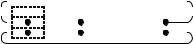
//Manipulations of entire lists
//( a, . . . , b , c, . . . , d ) → ( a, . . . , b, c, . . . , d , )
Procedure concat(L : List) splice(L .first, L .last, last)
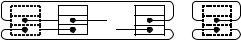
// a, . . . , b → |
|
|
|
|
|
|
Procedure makeEmpty |
··· |
|||||
freeList.concat(this ) |
// |
|
··· |
→ |
|
|
|
|
|
|
Fig. 3.5. More constant-time operations on doubly linked lists
Exercise 3.1 (alternative list implementation). Discuss an alternative implementation of List that does not need the dummy item h. Instead, this representation stores a pointer to the first list item in the list object. The position before the first list element is encoded as a null pointer. The interface and the asymptotic execution times of all operations should remain the same. Give at least one advantage and one disadvantage of this implementation compared with the one given in the text.
The dummy item is also useful for other operations. For example, consider the problem of finding the next occurrence of an element x starting at an item from. If x is not present, head should be returned. We use the dummy element as a sentinel. A sentinel is an element in a data structure that makes sure that some loop will terminate. In the case of a list, we store the key we are looking for in the dummy element. This ensures that x is present in the list structure and hence a search for it will always terminate. The search will terminate in a proper list item or the dummy item, depending on whether x was present in the list originally. It is no longer necessary, to test whether the end of the list has been reached. In this way, the trick of using the dummy item h as a sentinel saves one test in each iteration and significantly improves the efficiency of the search:
64 3 Representing Sequences by Arrays and Linked Lists
Function findNext(x : Element; from : Handle) : Handle |
|
|
|
|
|
|
|
|
|
|
||||||
h.e = x |
// Sentinel |
|
|
|
|
|
|
|
|
|
|
|
|
|
|
|
|
x |
|
|
|
|
|
|
|
|
|
|
|
||||
while from → e = x do |
|
|
|
|
|
|
|
|
|
|
||||||
|
|
|
|
|
|
|
|
|
||||||||
|
|
|
|
|
|
|
|
|
|
|
||||||
from := from → next |
|
|
|
|
|
|
|
|
··· |
··· |
|
|
|
|
|
|
|
|
|
|
|
|
|
|
|
|
|
|
|
|
|
||
|
|
|
|
|
|
|
|
|
|
|
|
|
|
|
||
return from
Exercise 3.2. Implement a procedure swap that swaps two sublists in constant time, i.e., sequences ( . . . , a , a, . . . , b, b , . . . , . . . , c , c, . . . , d, d , . . . ) are transformed into
( . . . , a , c, . . . , d, b , . . . , . . . , c , a, . . . , b, d , . . . ). Is splice a special case of swap?
Exercise 3.3 (memory management). Implement the function checkFreelist called by insertAfter in Fig. 3.5. Since an individual call of the programming-language primitive allocate for every single item might be too slow, your function should allocate space for items in large batches. The worst-case execution time of checkFreeList should be independent of the batch size. Hint: in addition to freeList, use a small array of free items.
Exercise 3.4. Give a constant-time implementation of an algorithm for rotating a list to the right: a, . . . , b, c → c, a, . . . , b . Generalize your algorithm to rotate
a, . . . , b, c, . . . , d to c, . . . , d, a, . . . , b in constant time.
Exercise 3.5. findNext using sentinels is faster than an implementation that checks for the end of the list in each iteration. But how much faster? What speed difference do you predict for many searches in a short list with 100 elements, and in a long list with 10 000 000 elements, respectively? Why is the relative speed difference dependent on the size of the list?
Maintaining the Size of a List
In our simple list data type, it is not possible to determine the length of a list in constant time. This can be fixed by introducing a member variable size that is updated whenever the number of elements changes. Operations that affect several lists now need to know about the lists involved, even if low-level functions such as splice only need handles to the items involved. For example, consider the following code for moving an element a from a list L to the position after a in a list L :
Procedure moveAfter(a, a : Handle; L, L : List) splice(a, a, a ); L.size--; L .size++
Maintaining the size of lists interferes with other list operations. When we move elements as above, we need to know the sequences containing them and, more seriously, operations that move sublists between lists cannot be implemented in constant time anymore. The next exercise offers a compromise.
Exercise 3.6. Design a list data type that allows sublists to be moved between lists in constant time and allows constant-time access to size whenever sublist operations have not been used since the last access to the list size. When sublist operations have been used, size is recomputed only when needed.
3.1 Linked Lists |
65 |
Exercise 3.7. Explain how the operations remove, insertAfter, and concat have to be modified to keep track of the length of a List.
3.1.2 Singly Linked Lists
The two pointers per item of a doubly linked list make programming quite easy. Singly linked lists are the lean sisters of doubly linked lists. We use SItem to refer to an item in a singly linked list. SItems scrap the predecessor pointer and store only a pointer to the successor. This makes singly linked lists more space-efficient and often faster than their doubly linked brothers. The downside is that some operations can no longer be performed in constant time or can no longer be supported in full generality. For example, we can remove an SItem only if we know its predecessor.
We adopt the implementation approach used with doubly linked lists. SItems form collections of cycles, and an SList has a dummy SItem h that precedes the first proper element and is the successor of the last proper element. Many operations on Lists can still be performed if we change the interface slightly. For example, the following implementation of splice needs the predecessor of the first element of the sublist to be moved:
// ( |
. . . |
, a , a, . . . , b, b . . |
. |
, |
|
. . . , t, t , . . . ) |
→ |
( |
. . . |
, a , b . . |
. , |
. . . , t, a, . . . , b, t , . . . ) |
|
|
|
|
|
|
|
|
Procedure splice(a ,b,t : SHandle) |
|
a |
a |
|
b b |
|
|||||
a |
next |
|
b |
next |
|
// |
|
|
··· |
|
|
t |
→next |
:= a |
→ next |
|
|
|
|
||||
|
→ |
|
|
→ |
|
|
|
|
|
|
|
|
|
|
|
|
|
|
|
|
|
||
b → next |
|
t → next |
|
|
t |
|
|
t |
|
||
Similarly, findNext should not return the handle of the SItem with the next hit but its predecessor, so that it remains possible to remove the element found. Consequently, findNext can only start searching at the item after the item given to it. A useful addition to SList is a pointer to the last element because it allows us to support pushBack in constant time.
Exercise 3.8. Implement classes SHandle, SItem, and SList for singly linked lists in analogy to Handle, Item, and List. Show that the following functions can be implemented to run in constant time. The operations head, first, last, isEmpty, popFront, pushFront, pushBack, insertAfter, concat, and makeEmpty should have the same interface as before. The operations moveAfter, moveToFront, moveToBack, remove, popFront, and findNext need different interfaces.
We shall see several applications of singly linked lists in later chapters, for example in hash tables in Sect. 4.1 and in mergesort in Sect. 5.2. We may also use singly linked lists to implement free lists of memory managers – even for items in doubly linked lists.
66 3 Representing Sequences by Arrays and Linked Lists
3.2 Unbounded Arrays
Consider an array data structure following operations pushBack,
that, besides the indexing operation [·], supports the popBack, and size:
e0, . . . , en .pushBack(e) = e0, . . . , en, e ,
e0, . . . , en .popBack = e0, . . . , en−1 , size( e0, . . . , en−1 ) = n .
Why are unbounded arrays important? Because in many situations we do not know in advance how large an array should be. Here is a typical example: suppose you want to implement the Unix command sort for sorting the lines of a file. You decide to read the file into an array of lines, sort the array internally, and finally output the sorted array. With unbounded arrays, this is easy. With bounded arrays, you would have to read the file twice: once to find the number of lines it contains, and once again to actually load it into the array.
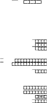
We come now to the implementation of unbounded arrays. We emulate an unbounded array u with n elements by use of a dynamically allocated bounded array b with w entries, where w ≥ n. The first n entries of b are used to store the elements of u. The last w − n entries of b are unused. As long as w > n, pushBack simply increments n and uses the first unused entry of b for the new element. When w = n, the next pushBack allocates a new bounded array b that is larger by a constant factor (say a factor of two). To reestablish the invariant that u is stored in b, the contents of b are copied to the new array so that the old b can be deallocated. Finally, the pointer defining b is redirected to the new array. Deleting the last element with popBack is even easier, since there is no danger that b may become too small. However, we might waste a lot of space if we allow b to be much larger than needed. The wasted space can be kept small by shrinking b when n becomes too small. Figure 3.6 gives the complete pseudocode for an unbounded-array class. Growing and shrinking are performed using the same utility procedure reallocate. Our implementation uses constants α and β , with β = 2 and α = 4. Whenever the current bounded array becomes too small, we replace it by an array of β times the old size. Whenever the size of the current array becomes α times as large as its used part, we replace it by an array of size β n. The reasons for the choice of α and β shall become clear later.
3.2.1 Amortized Analysis of Unbounded Arrays: The Global Argument
Our implementation of unbounded arrays follows the algorithm design principle “make the common case fast”. Array access with [·] is as fast as for bounded arrays. Intuitively, pushBack and popBack should “usually” be fast – we just have to update n. However, some insertions and deletions incur a cost of Θ (n). We shall show that such expensive operations are rare and that any sequence of m operations starting with an empty array can be executed in time O(m).
Lemma 3.1. Consider an unbounded array u that is initially empty. Any sequence σ = σ1, . . . , σm of pushBack or popBack operations on u is executed in time O(m).
|
3.2 |
Unbounded Arrays |
67 |
|||||||||||||||||||
Class UArray of Element |
|
|
|
|
|
|
|
|
|
|
|
|
|
|
|
|
|
|
|
|
|
|
Constant β = 2 : R+ |
|
|
|
|
|
|
|
|
|
|
|
|
|
// growth factor |
||||||||
Constant α = 4 : R+ |
|
|
|
|
|
|
// worst case memory blowup |
|||||||||||||||
w = 1 : N |
|
|
|
|
|
|
|
|
|
|
|
|
|
// allocated size |
||||||||
n = 0 : N |
|
|
|
|
|
|
|
|
|
|
|
|
|
|
// current size. |
|||||||
invariant n ≤ w < α n or n = 0 and w ≤ β |
|
|
|
|
|
|
|
|
|
|
|
n |
|
|
|
|
|
|
|
w |
||
b : Array [0..w − 1] of Element |
// b → |
e0 |
|
··· |
en−1 |
|
|
··· |
|
|
|
|
|
|
||||||||
Operator [i : N] : Element |
|
|
|
|
|
|
|
|
|
|
|
|
|
|
|
|
|
|
|
|
|
|
assert 0 ≤ i < n |
|
|
|
|
|
|
|
|
|
|
|
|
|
|
|
|
|
|
|
|
|
|
return b[i] |
|
|
|
|
|
|
|
|
|
|
|
|
|
|
|
|
|
|
|
|
|
|
Function size : N return n |
|
|
|
|
|
|
|
|
|
|
|
|
|
|
|
|
|
|
|
|
|
|
Procedure pushBack(e : Element) |
|
|
|
|
|
|
|
|
// Example for n = w = 4: |
|||||||||||||
if n = w then |
|
|
|
|
|
|
|
|
|
|
|
|
|
// b → |
|
|
|
|
|
|
||
|
|
|
|
|
|
|
|
|
|
|
|
|
|
0 |
1 |
2 |
3 |
|||||
reallocate(β n) |
|
|
|
|
|
|
|
|
// b → |
|
|
|
3 |
|
|
|
|
|
|
|||
|
|
|
|
|
|
|
|
0 |
1 |
2 |
|
|
|
|
|
|
||||||
b[n] := e |
|
|
|
|
|
|
|
|
// b → |
|
|
|
|
3 |
|
e |
|
|
|
|||
|
|
|
|
|
|
|
|
0 |
1 |
2 |
|
|
|
|
||||||||
n++ |
|
|
|
|
|
|
|
|
// b → |
|
|
|
3 e |
|
|
|
||||||
|
|
|
|
|
|
|
|
0 |
1 |
2 |
|
|
|
|||||||||
Procedure popBack |
|
|
|
|
|
// Example for n = 5, w = 16: |
||||||||||||||||
assert n > 0 |
// b → |
|
0 |
|
|
|
|
|
|
|
|
|
|
|
|
|
|
|||||
|
1 |
2 |
3 |
4 |
|
|
|
|
|
|
|
|
|
|
|
|
|
|
||||
n |
// b → |
|
0 |
|
|
4 |
|
|
|
|
|
|
|
|
|
|
||||||
|
1 |
2 |
3 |
|
|
|
|
|
|
|
|
|
|
|
|
|
|
|||||
-- |
|
|
|
|
|
|
|
|
|
|
|
|
|
|
|
|
|
|
|
|
|
|
if α n ≤ w n > 0 then |
|
|
|
|
|
|
|
|
|
// reduce waste of space |
||||||||||||
reallocate(β n) |
|
|
|
|
|
|
|
|
// b → |
|
3 |
|
|
|
|
|
||||||
|
|
|
|
|
|
|
|
|
0 |
1 |
2 |
|
|
|
|
|||||||
Procedure reallocate(w : N) |
|
|
|
|
|
|
// Example for w = 4, w = 8: |
|||||||||||||||
w := w |
|
|
|
|
|
|
|
|
|
|
|
|
|
// b → |
|
0 |
1 |
2 |
3 |
|||
b := allocate Array [0..w − 1] of Element |
|
// b → |
|
|
|
|
|
|
|
|
|
|||||||||||
(b [0], . . . , b [n − 1]) := (b[0], . . . , b[n − 1]) |
|
// b → 0 1 2 3 |
|
|
|
|||||||||||||||||
dispose b |
|
|
|
|
|
|
|
|
|
|
|
|
|
// b → 0 1 2 3 |
||||||||
b := b |
// pointer assignment b → |
|
0 |
|
1 |
2 |
3 |
|
|
|
|
|
|
|||||||||
Fig. 3.6. Pseudocode for unbounded arrays
Lemma 3.1 is a nontrivial statement. A small and innocent-looking change to the program invalidates it.
Exercise 3.9. Your manager asks you to change the initialization of α to α = 2. He argues that it is wasteful to shrink an array only when three-fourths of it are unused. He proposes to shrink it when n ≤ w/2. Convince him that this is a bad idea by giving a sequence of m pushBack and popBack operations that would need time Θ m2 if his proposal was implemented.
68 3 Representing Sequences by Arrays and Linked Lists
Lemma 3.1 makes a statement about the amortized cost of pushBack and popBack operations. Although single operations may be costly, the cost of a sequence of m operations is O(m). If we divide the total cost of the operations in σ by the number of operations, we get a constant. We say that the amortized cost of each operation is constant. Our usage of the term “amortized” is similar to its usage in everyday language, but it avoids a common pitfall. “I am going to cycle to work every day from now on, and hence it is justified to buy a luxury bike. The cost per ride will be very small – the investment will be amortized.” Does this kind of reasoning sound familiar to you? The bike is bought, it rains, and all good intentions are gone. The bike has not been amortized. We shall instead insist that a large expenditure is justified by savings in the past and not by expected savings in the future. Suppose your ultimate goal is to go to work in a luxury car. However, you are not going to buy it on your first day of work. Instead, you walk and put a certain amount of money per day into a savings account. At some point, you will be able to buy a bicycle. You continue to put money away. At some point later, you will be able to buy a small car, and even later you can finally buy a luxury car. In this way, every expenditure can be paid for by past savings, and all expenditures are amortized. Using the notion of amortized costs, we can reformulate Lemma 3.1 more elegantly. The increased elegance also allows better comparisons between data structures.
Corollary 3.2. Unbounded arrays implement the operation [·] in worst-case constant time and the operations pushBack and popBack in amortized constant time.
To prove Lemma 3.1, we use the bank account or potential method. We associate an account or potential with our data structure and force every pushBack and popBack to put a certain amount into this account. Usually, we call our unit of currency a token. The idea is that whenever a call of reallocate occurs, the balance in the account is sufficiently high to pay for it. The details are as follows. A token can pay for moving one element from b to b . Note that element copying in the procedure reallocate is the only operation that incurs a nonconstant cost in Fig. 3.6. More concretely, reallocate is always called with w = 2n and thus has to copy n elements. Hence, for each call of reallocate, we withdraw n tokens from the account. We charge two tokens for each call of pushBack and one token for each call of popBack. We now show that these charges suffice to cover the withdrawals made by reallocate.
The first call of reallocate occurs when there is one element already in the array and a new element is to be inserted. The element already in the array has deposited two tokens in the account, and this more than covers the one token withdrawn by reallocate. The new element provides its tokens for the next call of reallocate.
After a call of reallocate, we have an array of w elements: n = w/2 slots are occupied and w/2 are free. The next call of reallocate occurs when either n = w or 4n ≤ w. In the first case, at least w/2 elements have been added to the array since the last call of reallocate, and each one of them has deposited two tokens. So we have at least w tokens available and can cover the withdrawal made by the next call of reallocate. In the second case, at least w/2 − w/4 = w/4 elements have been removed from the array since the last call of reallocate, and each one of them has deposited one token. So we have at least w/4 tokens available. The call of reallocate
3.2 Unbounded Arrays |
69 |
needs at most w/4 tokens, and hence the cost of the call is covered. This completes the proof of Lemma 3.1.
Exercise 3.10. Redo the argument above for general values of α and β , and charge β /(β − 1) tokens for each call of pushBack and β /(α − β ) tokens for each call of popBack. Let n be such that w = β n . Then, after a reallocate, n elements are occupied and (β − 1)n = ((β − 1)/β )w are free. The next call of reallocate occurs when either n = w or α n ≤ w. Argue that in both cases there are enough tokens.
Amortized analysis is an extremely versatile tool, and so we think that it is worthwhile to know some alternative proof methods. We shall now give two variants of the proof above.
Above, we charged two tokens for each pushBack and one token for each popBack. Alternatively, we could charge three tokens for each pushBack and not charge popBack at all. The accounting is simple. The first two tokens pay for the insertion as above, and the third token is used when the element is deleted.
Exercise 3.11 (continuation of Exercise 3.10). Show that a charge of β /(β − 1) +
β /(α − β ) tokens for each pushBack is enough. Determine values of α such that β /(α − β ) ≤ 1/(β − 1) and β /(α − β ) ≤ β /(β − 1), respectively.
3.2.2 Amortized Analysis of Unbounded Arrays: The Local Argument
We now describe our second modification of the proof. In the argument above, we used a global argument in order to show that there are enough tokens in the account before each call of reallocate. We now show how to replace the global argument by a local argument. Recall that, immediately after a call of reallocate, we have an array of w elements, out of which w/2 are filled and w/2 are free. We argue that at any time after the first call of reallocate, the following token invariant holds:
the account contains at least max(2(n − w/2), w/2 − n) tokens.
Observe that this number is always nonnegative. We use induction on the number of operations. Immediately after the first reallocate, there is one token in the account and the invariant requires none. A pushBack increases n by one and adds two tokens. So the invariant is maintained. A popBack removes one element and adds one token. So the invariant is again maintained. When a call of reallocate occurs, we have either n = w or 4n ≤ w. In the former case, the account contains at least n tokens, and n tokens are required for the reallocation. In the latter case, the account contains at least w/4 tokens, and n are required. So, in either case, the number of tokens suffices. Also, after the reallocation, n = w/2 and hence no tokens are required.
Exercise 3.12. Charge three tokens for a pushBack and no tokens for a popBack. Argue that the account contains always at least n + max(2(n − w/2), w/2 − n) = max(3n − w, w/2) tokens.