

Algorithms and data structures
.pdf5.1 Simple Sorters |
101 |
Exercise 5.3 (a simple scheduling problem). A hotel manager has to process n advance bookings of rooms for the next season. His hotel has k identical rooms. Bookings contain an arrival date and a departure date. He wants to Þnd out whether there are enough rooms in the hotel to satisfy the demand. Design an algorithm that solves this problem in time O(n log n). Hint: consider the set of all arrivals and departures. Sort the set and process it in sorted order.
Exercise 5.4 (sorting with a small set of keys). Design an algorithm that sorts n elements in O(k log k + n) expected time if there are only k different keys appearing in the input. Hint: combine hashing and sorting.
Exercise 5.5 (checking). It is easy to check whether a sorting routine produces a sorted output. It is less easy to check whether the output is also a permutation of the input. But here is a fast and simple Monte Carlo algorithm for integers: (a) Show thate1, . . . , en is a permutation of e1, . . . , en iff the polynomial
n |
n |
q(z) := ∏(z − ei) − ∏(z − ei) |
|
i=1 |
i=1 |
is identically zero. Here, z is a variable. (b) For any ε > 0, let p be a prime with p > max {n/ε , e1, . . . , en, e1, . . . , en}. Now the idea is to evaluate the above polynomial mod p for a random value z [0.. p −1]. Show that if e1, . . . , en is not a permutation of e1, . . . , en , then the result of the evaluation is zero with probability at most ε . Hint: a nonzero polynomial of degree n has at most n zeros.
5.1 Simple Sorters
We shall introduce two simple sorting techniques here: selection sort and insertion sort.
Selection sort repeatedly selects the smallest element from the input sequence, deletes it, and adds it to the end of the output sequence. The output sequence is initially empty. The process continues until the input sequence is exhausted. For example,
, 4, 7, 1, 1 1 , 4, 7, 1 1, 1 , 4, 7 1, 1, 4 , 7 1, 1, 4, 7 , .
The algorithm can be implemented such that it uses a single array of n elements and works in-place, i.e., it needs no additional storage beyond the input array and a constant amount of space for loop counters, etc. The running time is quadratic.
Exercise 5.6 (simple selection sort). Implement selection sort so that it sorts an array with n elements in time O n2 by repeatedly scanning the input sequence. The algorithm should be in-place, i.e., the input sequence and the output sequence should share the same array. Hint: the implementation operates in n phases numbered 1 to n. At the beginning of the i-th phase, the Þrst i − 1 locations of the array contain the i − 1 smallest elements in sorted order and the remaining n − i + 1 locations contain the remaining elements in arbitrary order.

102 5 Sorting and Selection
In Sect. 6.5, we shall learn about a more sophisticated implementation where the input sequence is maintained as a priority queue. Priority queues support efÞcient repeated selection of the minimum element. The resulting algorithm runs in time O(n log n) and is frequently used. It is efÞcient, it is deterministic, it works in-place, and the input sequence can be dynamically extended by elements that are larger than all previously selected elements. The last feature is important in discrete-event simulations, where events are to be processed in increasing order of time and processing an event may generate further events in the future.
Selection sort maintains the invariant that the output sequence is sorted by carefully choosing the element to be deleted from the input sequence. Insertion sort maintains the same invariant by choosing an arbitrary element of the input sequence but taking care to insert this element at the right place in the output sequence. For example,
, 4, 7, 1, 1 4 , 7, 1, 1 4, 7 , 1, 1 1, 4, 7 , 1 1, 1, 4, 7 , .
Figure 5.1 gives an in-place array implementation of insertion sort. The implementation is straightforward except for a small trick that allows the inner loop to use only a single comparison. When the element e to be inserted is smaller than all previously inserted elements, it can be inserted at the beginning without further tests. Otherwise, it sufÞces to scan the sorted part of a from right to left while e is smaller than the current element. This process has to stop, because a[1] ≤ e.
In the worst case, insertion sort is quite slow. For example, if the input is sorted in decreasing order, each input element is moved all the way to a[1], i.e., in iteration i of the outer loop, i elements have to be moved. Overall, we obtain
n |
|
|
|
n |
|
n(n + 1) |
|
|
|
n(n − 1) |
|
|
∑ |
(i |
− |
1) = n + |
∑ |
i = |
|
− |
n = |
= Ω n2 |
|||
|
|
|||||||||||
|
− |
2 |
|
2 |
|
|||||||
i=2 |
|
|
|
i=1 |
|
|
|
|
|
|
|
|
movements of elements (see also (A.11)).
Nevertheless, insertion sort is useful. It is fast for small inputs (say, n ≤ 10) and hence can be used as the base case in divide-and-conquer algorithms for sorting.
Procedure insertionSort(a : Array [1..n] of Element) |
|
for i := 2 to n do |
|
invariant a[1] ≤ ··· ≤ a[i − 1] |
|
// move a[i] to the right place |
|
e := a[i] |
|
if e < a[1] then |
// new minimum |
for j := i downto 2 do a[ j] := a[ j − 1] |
|
a[1] := e |
|
else |
// use a[1] as a sentinel |
for j := i downto −∞ while a[ j − 1] > e do a[ j] := a[ j − 1] a[ j] := e
Fig. 5.1. Insertion sort
5.2 Mergesort Ð an O(n log n) Sorting Algorithm |
103 |
Furthermore, in some applications the input is already ÒalmostÓ sorted, and in this situation insertion sort will be fast.
Exercise 5.7 (almost sorted inputs). Prove that insertion sort runs in time O(n + D) where D = ∑i |r(ei) − i| and r(ei) is the rank (position) of ei in the sorted output.
Exercise 5.8 (average-case analysis). Assume that the input to an insertion sort is a permutation of the numbers 1 to n. Show that the average execution time over all possible permutations is Ω n2 . Hint: argue formally that about one-third of the input elements in the right third of the array have to be moved to the left third of the array. Can you improve the argument to show that, on average, n2/4 − O(n) iterations of the inner loop are needed?
Exercise 5.9 (insertion sort with few comparisons). Modify the inner loops of the array-based insertion sort algorithm in Fig. 5.1 so that it needs only O(n log n) comparisons between elements. Hint: use binary search as discussed in Chap. 7. What is the running time of this modiÞcation of insertion sort?
Exercise 5.10 (efficient insertion sort?). Use the data structure for sorted sequences described in Chap. 7 to derive a variant of insertion sort that runs in time O(n log n).
*Exercise 5.11 (formal verification). Use your favorite veriÞcation formalism, for example Hoare calculus, to prove that insertion sort produces a permutation of the input (i.e., it produces a sorted permutation of the input).
5.2 Mergesort – an O(n log n) Sorting Algorithm
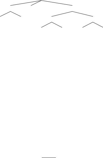
Mergesort is a straightforward application of the divide-and-conquer principle. The unsorted sequence is split into two parts of about equal size. The parts are sorted recursively, and the sorted parts are merged into a single sorted sequence. This approach is efÞcient because merging two sorted sequences a and b is quite simple. The globally smallest element is either the Þrst element of a or the Þrst element of b. So we move the smaller element to the output, Þnd the second smallest element using the same approach, and iterate until all elements have been moved to the output. Figure 5.2 gives pseudocode, and Figure 5.3 illustrates a sample execution. If the sequences are represented as linked lists (see, Sect. 3.1), no allocation and deallocation of list items is needed. Each iteration of the inner loop of merge performs one element comparison and moves one element to the output. Each iteration takes constant time. Hence, merging runs in linear time.
Theorem 5.1. The function merge, applied to sequences of total length n, executes in time O(n) and performs at most n − 1 element comparisons.
For the running time of mergesort, we obtain the following result.
Theorem 5.2. Mergesort runs in time O(n log n) and performs no more than n log n
element comparisons.
104 5 Sorting and Selection
Function mergeSort( e1, . . . , en ) : Sequence of Element if n = 1 then return e1
else return merge( mergeSort( e1, . . . , e n/2 ), mergeSort( e n/2 +1, . . . , en ))
// merging two sequences represented as lists |
|
|
|
|
|||||
Function merge(a, b : Sequence of Element) : Sequence of Element |
|
||||||||
c := |
|
|
|
|
|
|
|
|
|
loop |
|
|
|
|
|
|
|
|
|
|
invariant a, b, and c are sorted and e c, e a b : e ≤ e |
|
|||||||
|
if a.isEmpty |
then |
c.concat(b); return c |
|
|
|
|||
|
if b.isEmpty |
then |
c.concat(a); return c |
|
|
|
|||
|
if a.first ≤ b.first then |
c.moveToBack(a.first) |
|
|
|
||||
|
else |
|
c.moveToBack(b.first) |
|
|
|
|||
|
|
|
|
Fig. 5.2. Mergesort |
|
|
|
||
split |
2, 7, 1, 8, 2, 8, 1 |
|
|
a |
b |
|
c |
operation |
|
|
|
|
|||||||
|
2, 7, 1 |
8, 2, 8, 1 |
|
|
|||||
|
|
|
|
|
|
|
|||
split |
1, 2, 7 1, 2, 8, 8 |
|
|
move a |
|||||
|
|
|
|
||||||
split |
2 7, 1 |
8, 2 |
8, 1 |
2, 7 |
1, 2, 8, 8 |
|
1 |
move b |
|
|
7 1 8 2 8 1 |
2, 7 2, 8, 8 |
|
1, 1 |
move a |
||||
merge |
7 |
2, 8, 8 |
|
1, 1, 2 |
move b |
||||
|
1, 7 |
2, 8 1, 8 |
7 |
8, 8 |
|
1, 1, 2, 2 |
move a |
||
merge |
1, 2, 7 |
1, 2, 8, 8 |
|
|
8, 8 |
|
1, 1, 2, 2, 7 |
concat b |
|
merge |
|
|
|
1, 1, 2, 2, 7, 8, 8 |
|
||||
|
|
||||||||
|
1, 1, 2, 2, 7, 8, 8 |
|
|
|
|
|
|
|
|
Fig. 5.3. Execution of mergeSort( 2, 7, 1, 8, 2, 8, 1 ). The left part illustrates the recursion in mergeSort and the right part illustrates the merge in the outermost call
Proof. Let C(n) denote the worst-case number of element comparisons performed. We have C(1) = 0 and C(n) ≤ C( n/2 ) +C( n/2 ) + n −1, using Theorem 5.1. The master theorem for recurrence relations (2.5) suggests that C(n) = O(n log n). We shall give two proofs. The Þrst proof shows that C(n) ≤ 2n log n , and the second proof shows that C(n) ≤ n log n .
For n a power of two, we deÞne D(1) = 0 and D(n) = 2D(n/2) + n. Then D(n) =
n log n for n a power of two, by the master theorem for recurrence relations. We claim that C(n) ≤ D(2k), where k is such that 2k−1 < n ≤ 2k. Then C(n) ≤ D(2k) = 2kk ≤
2n log n . It remains to argue the inequality C(n) ≤ D(2k). We use induction on k. For k = 0, we have n = 1 and C(1) = 0 = D(1), and the claim certainly holds. For k > 1, we observe that n/2 ≤ n/2 ≤ 2k−1, and hence
C(n) ≤ C( n/2 ) + C( n/2 ) + n − 1 ≤ 2D(2k−1) + 2k − 1 ≤ D(2k) .
This completes the Þrst proof. We turn now to the second, reÞned proof. We prove that
5.2 Mergesort Ð an O(n log n) Sorting Algorithm |
105 |
C(n) ≤ n log n − 2 log n + 1 ≤ n log n
by induction over n. For n = 1, the claim is certainly true. So, assume n > 1. We distinguish two cases. Assume Þrst that we have 2k−1 < n/2 ≤ n/2 ≤ 2k for some integer k. Then log n/2 = log n/2 = k and log n = k + 1, and hence
C(n) ≤ C( n/2 ) + C( n/2 ) + n − 1
≤n/2 k − 2k + 1 + n/2 k − 2k + 1 + n − 1
=nk + n − 2k+1 + 1 = n(k + 1) − 2k+1 + 1 = n log n − 2 log n + 1 .
Otherwise, we have n/2 = 2k−1 and n/2 = 2k−1 + 1 for some integer k, and therefore log n/2 = k − 1, log n/2 = k, and log n = k + 1. Thus
C(n) ≤ C( n/2 ) + C( n/2 ) + n − 1
≤ 2k−1(k − 1) − 2k−1 + 1 + (2k−1 + 1)k − 2k + 1 + 2k + 1 − 1
=(2k + 1)k − 2k−1 − 2k−1 + 1 + 1
=(2k + 1)(k + 1) − 2k+1 + 1 = n log n − 2 log n + 1 .
The bound for the execution time can be veriÞed using a similar recurrence relation.
Mergesort is the method of choice for sorting linked lists and is therefore frequently used in functional and logical programming languages that have lists as their primary data structure. In Sect. 5.3, we shall see that mergesort is basically optimal as far as the number of comparisons is concerned; so it is also a good choice if comparisons are expensive. When implemented using arrays, mergesort has the additional advantage that it streams through memory in a sequential way. This makes it efÞcient in memory hierarchies. Section 5.7 has more on that issue. Mergesort is still not the usual method of choice for an efÞcient array-based implementation, however, since merge does not work in-place. (But see Exercise 5.17 for a possible way out.)
Exercise 5.12. Explain how to insert k new elements into a sorted list of size n in time O(k log k + n).
Exercise 5.13. We discussed merge for lists but used abstract sequences for the description of mergeSort. Give the details of mergeSort for linked lists.
Exercise 5.14. Implement mergesort in a functional programming language.
Exercise 5.15. Give an efÞcient array-based implementation of mergesort in your favorite imperative programming language. Besides the input array, allocate one auxiliary array of size n at the beginning and then use these two arrays to store all intermediate results. Can you improve the running time by switching to insertion sort for small inputs? If so, what is the optimal switching point in your implementation?
106 5 Sorting and Selection
Exercise 5.16. The way we describe merge, there are three comparisons for each loop iteration Ð one element comparison and two termination tests. Develop a variant using sentinels that needs only one termination test. Can you do this task without appending dummy elements to the sequences?
Exercise 5.17. Exercise 3.20 introduced a list-of-blocks representation for sequences. Implement merging and mergesort for this data structure. During merging, reuse emptied input blocks for the output sequence. Compare the space and time efÞciency of mergesort for this data structure, for plain linked lists, and for arrays. Pay attention to constant factors.
5.3 A Lower Bound
Algorithms give upper bounds on the complexity of a problem. By the preceding discussion, we know that we can sort n items in time O(n log n). Can we do better, and maybe even achieve linear time? A ÒyesÓ answer requires a better algorithm and its analysis. But how could we potentially argue a ÒnoÓ answer? We would have to argue that no algorithm, however ingenious, can run in time o(n log n). Such an argument is called a lower bound. So what is the answer? The answer is both no and yes. The answer is no, if we restrict ourselves to comparison-based algorithms, and the answer is yes if we go beyond comparison-based algorithms. We shall discuss non-comparison-based sorting in Sect. 5.6.
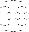
So what is a comparison-based sorting algorithm? The input is a set {e1, . . . , en} of n elements, and the only way the algorithm can learn about its input is by comparing elements. In particular, it is not allowed to exploit the representation of keys, for example as bit strings. Deterministic comparison-based algorithms can be viewed as trees. They make an initial comparison; for instance, the algorithms asks Òei ≤ e j?Ó, with outcomes yes and no. On the basis of the outcome, the algorithm proceeds to the next comparison. The key point is that the comparison made next depends only on the outcome of all preceding comparisons and nothing else. Figure 5.4 shows a sorting tree for three elements.
When the algorithm terminates, it must have collected sufÞcient information so that it can commit to a permutation of the input. When can it commit? We perform the following thought experiment. We assume that the input keys are distinct, and consider any of the n! permutations of the input, say π . The permutation π corresponds to the situation that eπ (1) < eπ (2) < . . . < eπ (n). We answer all questions posed by the algorithm so that they conform to the ordering deÞned by π . This will lead us to a leaf π of the comparison tree.
Lemma 5.3. Let π and σ be two distinct permutations of n elements. The leaves π and σ must then be distinct.
Proof. Assume otherwise. In a leaf, the algorithm commits to some ordering of the input and so it cannot commit to both π and σ . Say it commits to π . Then, on an input ordered according to σ , the algorithm is incorrect, which is a contradiction.
5.3 A Lower Bound |
107 |
The lemma above tells us that any comparison tree for sorting must have at least n! leaves. Since a tree of depth T has at most 2T leaves, we must have
2T ≥ n! or T ≥ log n! .
Via StirlingÕs approximation to the factorial (A.9), we obtain
n n |
|
T ≥ log n! ≥ log e |
= n log n − n log e . |
Theorem 5.4. Any comparison-based sorting algorithm needs n log n − O(n) comparisons in the worst case.
We state without proof that this bound also applies to randomized sorting algorithms and to the average-case complexity of sorting, i.e., worst-case instances are not much more difÞcult than random instances. Furthermore, the bound applies even if we only want to solve the seemingly simpler problem of checking whether some element appears twice in a sequence.
Theorem 5.5. Any comparison-based sorting algorithm needs n log n − O(n) comparisons on average, i.e.,
∑π dπ = n log n − O(n) ,
n!
where the sum extends over all n! permutations of the n elements and dπ is the depth of the leaf π .
Exercise 5.18. Show that any comparison-based algorithm for determining the smallest of n elements requires n − 1 comparisons. Show also that any comparison-based algorithm for determining the smallest and second smallest elements of n elements requires at least n −1 + log n comparisons. Give an algorithm with this performance.
|
e1?e2 |
|
|
|
≤ |
> |
|
e2?e3 |
e2?e3 |
||
≤ |
> |
≤ |
> |
|
|||
e1 ≤ e2 ≤ e3 |
e1?e3 > |
e1?e3 |
e1 > e2 > e3 |
≤ |
|
≤ |
> |
e1 ≤ e3 < e2 |
e3 < e1 ≤ e2 |
e2 < e1 ≤ e3 |
e2 ≤ e3 < e1 |
Fig. 5.4. A tree that sorts three elements. We Þrst compare e1 and e2. If e1 ≤ e2, we compare e2 with e3. If e2 ≤ e3, we have e1 ≤ e2 ≤ e3 and are Þnished. Otherwise, we compare e1 with e3. For either outcome, we are Þnished. If e1 > e2, we compare e2 with e3. If e2 > e3, we have e1 > e2 > e3 and are Þnished. Otherwise, we compare e1 with e3. For either outcome, we are Þnished. The worst-case number of comparisons is three. The average number is (2 + 3 + 3 + 2 + 3 + 3)/6 = 8/3
108 5 Sorting and Selection
Exercise 5.19. The element uniqueness problem is the task of deciding whether in a set of n elements, all elements are pairwise distinct. Argue that comparison-based algorithms require Ω(n log n) comparisons. Why does this not contradict the fact that we can solve the problem in linear expected time using hashing?
Exercise 5.20 (lower bound for average case). With the notation above, let dπ be the depth of the leaf π . Argue that A = (1/n!) ∑π dπ is the average-case complexity of a comparison-based sorting algorithm. Try to show that A ≥ log n!. Hint: prove Þrst that ∑π 2−dπ ≤ 1. Then consider the minimization problem Òminimize ∑π dπ subject to ∑π 2−dπ ≤ 1Ó. Argue that the minimum is attained when all diÕs are equal.
Exercise 5.21 (sorting small inputs optimally). Give an algorithm for sorting k elements using at most log k! element comparisons. (a) For k {2, 3, 4}, use mergesort. (b) For k = 5, you are allowed to use seven comparisons. This is difÞcult. Mergesort does not do the job, as it uses up to eight comparisons. (c) For k {6, 7, 8}, use the case k = 5 as a subroutine.
5.4 Quicksort
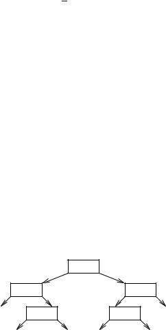
Quicksort is a divide-and-conquer algorithm that is complementary to the mergesort algorithm of Sect. 5.2. Quicksort does all the difÞcult work before the recursive calls. The idea is to distribute the input elements into two or more sequences that represent nonoverlapping ranges of key values. Then, it sufÞces to sort the shorter sequences recursively and concatenate the results. To make the duality to mergesort complete, we would like to split the input into two sequences of equal size. Unfortunately, this is a nontrivial task. However, we can come close by picking a random splitter element. The splitter element is usually called the pivot. Let p denote the pivot element chosen. Elements are classiÞed into three sequences a, b, and c of elements that are smaller than, equal to, or larger than p, respectively. Figure 5.5 gives a high-level realization of this idea, and Figure 5.6 depicts a sample execution. Quicksort has an expected execution time of O(n log n), as we shall show in Sect. 5.4.1. In Sect. 5.4.2, we discuss reÞnements that have made quicksort the most widely used sorting algorithm in practice.
Function quickSort(s : Sequence of Element) : Sequence of Element |
|
if |s| ≤ 1 then return s |
// base case |
pick p s uniformly at random |
// pivot key |
a := e s : e < p |
|
b := e s : e = p |
|
c := e s : e > p |
|
return concatenation of quickSort(a), b, and quickSort(c) |
|
Fig. 5.5. High-level formulation of quicksort for lists
|
|
|
|
|
|
|
5.4 Quicksort |
109 |
|
|
|
3, 6, 8, 1, 0, 7, 2, 4, 5, 9 |
|
|
|
|
|
||
1, 0, 2 |
3 |
6, 8, 7, 4, 5, 9 |
|
|
|
||||
|
|
2 |
4, 5 |
|
|
8, 7, 9 |
|
||
0 1 |
6 |
|
|||||||
|
|
|
|
|
7 |
|
|
|
|
|
|
4 5 |
8 9 |
|
|||||
Fig. 5.6. Execution of quickSort (Fig. 5.5) on 3, 6, 8, 1, 0, 7, 2, 4, 5, 9 using the Þrst element of a subsequence as the pivot. The Þrst call of quicksort uses 3 as the pivot and generates the subproblems 1, 0, 2 , 3 , and 6, 8, 7, 4, 5, 9 . The recursive call for the third subproblem uses 6 as a pivot and generates the subproblems 4, 5 , 6 , and 8, 7, 9
5.4.1 Analysis
To analyze the running time of quicksort for an input sequence s = e1, . . . , en , we focus on the number of element comparisons performed. We allow three-way comparisons here, with possible outcomes ÒsmallerÓ, ÒequalÓ, and ÒlargerÓ. Other operations contribute only constant factors and small additive terms to the execution time.
Let C(n) denote the worst-case number of comparisons needed for any input sequence of size n and any choice of pivots. The worst-case performance is easily determined. The subsequences a, b, and c in Fig. 5.5 are formed by comparing the pivot with all other elements. This makes n − 1 comparisons. Assume there are k elements smaller than the pivot and k elements larger than the pivot. We obtain
C(0) = C(1) = 0 and
C(n) ≤ n − 1 + max C(k) + C(k ) : 0 ≤ k ≤ n − 1, 0 ≤ k < n − k .
It is easy to verify by induction that
C(n) ≤ n(n − 1) = Θ n2 .
2
The worst case occurs if all elements are different and we always pick the largest or smallest element as the pivot. Thus C(n) = n(n − 1)/2.
The expected performance is much better. We Þrst argue for an O(n log n) bound and then show a bound of 2n ln n. We concentrate on the case where all elements are different. Other cases are easier because a pivot that occurs several times results in a larger middle sequence b that need not be processed any further. Consider a Þxed element ei, and let Xi denote the total number of times ei is compared with a pivot element. Then ∑i Xi is the total number of comparisons. Whenever ei is compared with a pivot element, it ends up in a smaller subproblem. Therefore, Xi ≤ n − 1, and we have another proof for the quadratic upper bound. Let us call a comparison ÒgoodÓ for ei if ei moves to a subproblem of at most three-quarters the size. Any ei

110 5 Sorting and Selection
can be involved in at most log4/3 n good comparisons. Also, the probability that a pivot which is good for ei is chosen, is at least 1/2; this holds because a bad pivot must belong to either the smallest or the largest quarter of the elements. So E[Xi] ≤ 2 log4/3 n, and hence E[∑i Xi] = O(n log n). We shall now give a different argument and a better bound.
Theorem 5.6. The expected number of comparisons performed by quicksort is
ø ≤ ≤
C(n) 2n ln n 1.45n logn .
Proof. Let s = e1, . . . , en denote the elements of the input sequence in sorted order. Elements ei and e j are compared at most once, and only if one of them is picked as a pivot. Hence, we can count comparisons by looking at the indicator random variables Xi j, i < j, where Xi j = 1 if ei and e j are compared and Xi j = 0 otherwise. We obtain
ø |
n |
n |
n |
n |
n |
n |
C(n) = E |
∑ ∑ Xi j |
= ∑ ∑ |
E[Xi j] = ∑ ∑ prob(Xi j = 1) . |
|||
|
i=1 j=i+1 |
i=1 j=i+1 |
i=1 j=i+1 |
|||
The middle transformation follows from the linearity of expectations (A.2). The last equation uses the deÞnition of the expectation of an indicator random variable
ø
E[Xi j] = prob(Xi j = 1). Before we can further simplify the expression for C(n), we need to determine the probability of Xi j being 1.
2
Lemma 5.7. For any i < j, prob(Xi j = 1) = j − i + 1 .
Proof. Consider the j −i + 1-element set M = {ei, . . . , e j}. As long as no pivot from M is selected, ei and e j are not compared, but all elements from M are passed to the same recursive calls. Eventually, a pivot p from M is selected. Each element in M has
| |
M |
| |
|
|
|
|
|
i |
j |
we have Xi j = 1. The |
|
the same chance 1/ |
|
of being selected. If p = e |
or p = e |
||||||||
|
|
|
| |
M |
| |
= 2/( j |
− |
|
|
i |
j |
probability for this event is 2/ |
|
|
i + 1). Otherwise, e |
and e are passed to |
|||||||
different recursive calls, so that they will never be compared. |
|
|
|||||||||
Now we can Þnish proving Theorem 5.6 using relatively simple calculations:
ø |
n |
n |
|
|
|
|
|
n |
n |
2 |
|
n n−i+1 |
2 |
|
|
C(n) = ∑ ∑ prob(Xi j |
= 1) = ∑ ∑ |
|
|
= ∑ ∑ |
|
|
|||||||||
j − i + 1 |
k |
||||||||||||||
|
i=1 j=i+1 |
|
|
|
i=1 j=i+1 |
i=1 k=2 |
|||||||||
|
n |
n |
2 |
|
n |
|
1 |
|
|
|
|
|
|
|
|
|
≤ ∑ ∑ |
|
= 2n ∑ |
|
= 2n(Hn − 1) ≤ 2n(1 + ln n − 1) = 2n ln n . |
||||||||||
|
k |
k |
|||||||||||||
|
i=1 k=2 |
|
|
k=2 |
|
|
|
|
|
|
|
|
|
||
For the last three steps, recall the properties of the n-th harmonic number Hn := ∑nk=1 1/k ≤ 1 + ln n (A.12).
Note that the calculations in Sect. 2.8 for left-to-right maxima were very similar, although we had quite a different problem at hand.