

Algorithms and data structures
.pdf50 2 Introduction
their bidirected counterparts, and so this section will concentrate on directed graphs and only mention undirected graphs when there is something special about them. For example, the number of edges of an undirected graph is only half the number of edges of its bidirected counterpart. Nodes of an undirected graph have identical indegree and outdegree, and so we simply talk about their degree. Undirected graphs are important because directions often do not matter and because many problems are
easier to solve (or even to deÞne) for undirected graphs than for general digraphs. A graph G = (V , E ) is a subgraph of G if V V and E E. Given G = (V, E)
and a subset V V , the subgraph induced by V is deÞned as G |
= (V , E ∩ (V × |
||||||||
V )). In Fig. 2.7, the node set |
{ |
v, w |
} |
in G induces the subgraph H = ( |
{ |
} |
, |
{ |
} |
|
|
v, w |
|
|
(v, w) ). |
||||
A subset E E of edges induces the subgraph (V, E ). |
|
|
|
|
|
||||
Often, additional information is associated with nodes or edges. In particular, we shall often need edge weights or costs c : E → R that map edges to some numeric value. For example, the edge (z, w) in graph G in Fig. 2.7 has a weight c((z, w)) = −2. Note that an edge {u, v} of an undirected graph has a unique edge weight, whereas, in a bidirected graph, we can have c((u, v)) = c((v, u)).
We have now seen quite many deÞnitions on one page of text. If you want to see them at work, you may jump to Chap. 8 to see algorithms operating on graphs. But things are also becoming more interesting here.
An important higher-level graph-theoretic concept is the notion of a path. A path p = v0, . . . , vk is a sequence of nodes in which consecutive nodes are connected by edges in E, i.e., (v0, v1) E, (v1, v2) E, . . . , (vk−1, vk) E; p has length k and runs from v0 to vk. Sometimes a path is also represented by its sequence of edges. For example, u, v, w = (u, v), (v, w) is a path of length 2 in Fig. 2.7. A path is simple if its nodes, except maybe for v0 and vk, are pairwise distinct. In Fig. 2.7,z, w, x, u, v, w, x, y is a nonsimple path.
Cycles are paths with a common Þrst and last node. A simple cycle visiting all nodes of a graph is called a Hamiltonian cycle. For example, the cycles, t, u, v, w, x, y, z, s in graph G in Fig. 2.7 is Hamiltonian. A simple undirected cycle contains at least three nodes, since we also do not allow edges to be used twice in simple undirected cycles.
The concepts of paths and cycles help us to deÞne even higher-level concepts. A digraph is strongly connected if for any two nodes u and v there is a path from u to v. Graph G in Fig. 2.7 is strongly connected. A strongly connected component of a digraph is a maximal node-induced strongly connected subgraph. If we remove edge (w, x) from G in Fig. 2.7, we obtain a digraph without any directed cycles. A digraph without any cycles is called a directed acyclic graph (DAG). In a DAG, every strongly connected component consists of a single node. An undirected graph is connected if the corresponding bidirected graph is strongly connected. The connected components are the strongly connected components of the corresponding bidirected graph. For example, graph U in Fig. 2.7 has connected components {u, v, w}, {s, t}, and {x}. The node set {u, w} induces a connected subgraph, but it is not maximal and hence not a component.
2.9 Graphs |
51 |
Exercise 2.17. Describe 10 substantially different applications that can be modeled using graphs; car and bicycle networks are not considered substantially different. At least Þve should be applications not mentioned in this book.
Exercise 2.18. A planar graph is a graph that can be drawn on a sheet of paper such that no two edges cross each other. Argue that street networks are not necessarily planar. Show that the graphs K5 and K33 in Fig. 2.7 are not planar.
2.9.1 A First Graph Algorithm
It is time for an example algorithm. We shall describe an algorithm for testing whether a directed graph is acyclic. We use the simple observation that a node v with outdegree zero cannot appear in any cycle. Hence, by deleting v (and its incoming edges) from the graph, we obtain a new graph G that is acyclic if and only if G is acyclic. By iterating this transformation, we either arrive at the empty graph, which is certainly acyclic, or obtain a graph G where every node has an outdegree of at least one. In the latter case, it is easy to Þnd a cycle: start at any node v and construct a path by repeatedly choosing an arbitrary outgoing edge until you reach a node v that you have seen before. The constructed path will have the form (v, . . . , v , . . . , v ), i.e., the part (v , . . . , v ) forms a cycle. For example, in Fig. 2.7, graph G has no node with outdegree zero. To Þnd a cycle, we might start at node z and follow the pathz, w, x, u, v, w until we encounter w a second time. Hence, we have identiÞed the cycle w, x, u, v, w . In contrast, if the edge (w, x) is removed, there is no cycle. Indeed, our algorithm will remove all nodes in the order w, v, u, t, s, z, y, x. In Chap. 8, we shall see how to represent graphs such that this algorithm can be implemented to run in linear time. See also Exercise 8.3. We can easily make our algorithm certifying. If the algorithm Þnds a cycle, the graph is certainly cyclic. If the algorithm reduces the graph to the empty graph, we number the nodes in the order in which they are removed from G. Since we always remove a node v of outdegree zero from the current graph, any edge out of v in the original graph must go to a node that was removed previously and hence has received a smaller number. Thus the ordering proves acyclicity: along any edge, the node numbers decrease.
Exercise 2.19. Show an n-node DAG that has n(n − 1)/2 edges.
2.9.2 Trees
An undirected graph is a tree if there is exactly one path between any pair of nodes; see Fig. 2.8 for an example. An undirected graph is a forest if there is at most one path between any pair of nodes. Note that each component of a forest is a tree.
Lemma 2.8. The following properties of an undirected graph G are equivalent:
1.G is a tree.
2.G is connected and has exactly n − 1 edges.
3.G is connected and contains no cycles.
52 2 Introduction
undirected undirected rooted
s |
|
t |
r |
|
|
|
|
|
|
||
|
r |
s |
t |
u |
s |
|
|
||||
u |
|
v |
|
v |
|
|
|
|
|
|
directed expression
r |
|
|
r |
|
+ |
|
t |
u |
s |
t |
u |
a |
/ |
|
v |
|
rooted v |
2 |
b |
|
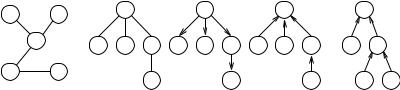
Fig. 2.8. Different kinds of trees. From left to right, we see an undirected tree, an undirected rooted tree, a directed out-tree, a directed in-tree, and an arithmetic expression
Proof. In a tree, there is a unique path between any two nodes. Hence the graph is connected and contains no cycles. Conversely, if there are two nodes that are connected by more than one path, the graph contains a cycle. Thus (1) and (3) are equivalent. We next show the equivalence of (2) and (3). Assume that G = (V, E) is connected, and let m = |E|. We perform the following experiment: we start with the empty graph and add the edges in E one by one. Addition of an edge can reduce the number of connected components by at most one. We start with n components and must end up with one component. Thus m ≥ n − 1. Assume now that there is an edge e = {u, v} whose addition does not reduce the number of connected components. Then u and v are already connected by a path, and hence addition of e creates a cycle. If G is cycle-free, this case cannot occur, and hence m = n − 1. Thus (3) implies (2). Assume next that G is connected and has exactly n − 1 edges. Again, add the edges one by one and assume that adding e = {u, v} creates a cycle. Then u and v are already connected, and hence e does not reduce the number of connected components. Thus (2) implies (3).
Lemma 2.8 does not carry over to digraphs. For example, a DAG may have many more than n − 1 edges. A directed graph is an out-tree with a root node r, if there is exactly one path from r to any other node. It is an in-tree with a root node r if there is exactly one path from any other node to r. Figure 2.8 shows examples. The depth of a node in a rooted tree is the length of the path to the root. The height of a rooted tree is the maximum over the depths of its nodes.
We can also make an undirected tree rooted by declaring one of its nodes to be the root. Computer scientists have the peculiar habit of drawing rooted trees with the root at the top and all edges going downwards. For rooted trees, it is customary to denote relations between nodes by terms borrowed from family relations. Edges go between a unique parent and its children. Nodes with the same parent are siblings. Nodes without children are leaves. Nonroot, nonleaf nodes are interior nodes. Consider a path such that u is between the root and another node v. Then u is an ancestor of v, and v is a descendant of u. A node u and its descendants form a subtree rooted at u. For example, in Fig. 2.8, r is the root; s, t, and v are leaves; s, t, and u are siblings because they are children of the same parent r; u is an interior node; r and u are ancestors of v; s, t, u, and v are descendants of r; and v and u form a subtree rooted at u.
|
|
2.10 P and NP |
53 |
Function eval(r) : R |
|
|
|
if r is a leaf then return the number stored in r |
|
|
|
else |
|
// r is an operator node |
|
v1 |
:= eval(first child of r) |
|
|
v2 |
:= eval(second child of r) |
|
|
return v1operator(r)v2 |
// apply the operator stored in r |
||
Fig. 2.9. Recursive evaluation of an expression tree rooted at r
2.9.3 Ordered Trees
Trees are ideally suited to representing hierarchies. For example, consider the expression a + 2/b. We have learned that this expression means that a and 2/b are added. But deriving this from the sequence of characters a, +, 2, /, b is difÞcult. For example, it requires knowledge of the rule that division binds more tightly than addition. Therefore compilers isolate this syntactical knowledge in parsers that produce a more structured representation based on trees. Our example would be transformed into the expression tree given in Fig. 2.8. Such trees are directed and, in contrast to graph-theoretic trees, they are ordered. In our example, a is the Þrst, or left, child of the root, and / is the right, or second, child of the root.
Expression trees are easy to evaluate by a simple recursive algorithm. Figure 2.9 shows an algorithm for evaluating expression trees whose leaves are numbers and whose interior nodes are binary operators (say +, −, ·, /).
We shall see many more examples of ordered trees in this book. Chapters 6 and 7 use them to represent fundamental data structures, and Chapter 12 uses them to systematically explore solution spaces.
2.10 P and NP
When should we call an algorithm efÞcient? Are there problems for which there is no efÞcient algorithm? Of course, drawing the line between ÒefÞcientÓ and ÒinefÞcientÓ is a somewhat arbitrary business. The following distinction has proved useful: an algorithm A runs in polynomial time, or is a polynomial-time algorithm, if there is a polynomial p(n) such that its execution time on inputs of size n is O(p(n)). If not otherwise mentioned, the size of the input will be measured in bits. A problem can be solved in polynomial time if there is a polynomial-time algorithm that solves it. We equate ÒefÞciently solvableÓ with Òpolynomial-time solvableÓ. A big advantage of this deÞnition is that implementation details are usually not important. For example, it does not matter whether a clever data structure can accelerate an O n3 algorithm by a factor of n. All chapters of this book, except for Chap. 12, are about efÞcient algorithms.
There are many problems for which no efÞcient algorithm is known. Here, we mention only six examples:
54 2 Introduction
•The Hamiltonian cycle problem: given an undirected graph, decide whether it contains a Hamiltonian cycle.
•The Boolean satisÞability problem: given a Boolean expression in conjunctive form, decide whether it has a satisfying assignment. A Boolean expression in
conjunctive form is a conjunction C1 C2 . . . Ck of clauses. A clause is a disjunction 1 2 . . . h of literals, and a literal is a variable or a negated variable. For example, v1 ¬v3 ¬v9 is a clause.
•The clique problem: given an undirected graph and an integer k, decide whether the graph contains a complete subgraph (= a clique) on k nodes.
•The knapsack problem: given n pairs of integers (wi, pi) and integers M and P, decide whether there is a subset I [1..n] such that ∑i I wi ≤ M and ∑i I pi ≥ P.
•The traveling salesman problem: given an edge-weighted undirected graph and an integer C, decide whether the graph contains a Hamiltonian cycle of length at most C. See Sect. 11.6.2 for more details.
•The graph coloring problem: given an undirected graph and an integer k, decide whether there is a coloring of the nodes with k colors such that any two adjacent nodes are colored differently.
The fact that we know no efÞcient algorithms for these problems does not imply that none exists. It is simply not known whether an efÞcient algorithm exists or not. In particular, we have no proof that such algorithms do not exist. In general, it is very hard to prove that a problem cannot be solved in a given time bound. We shall see some simple lower bounds in Sect. 5.3. Most algorithmicists believe that the six problems above have no efÞcient solution.
Complexity theory has found an interesting surrogate for the absence of lowerbound proofs. It clusters algorithmic problems into large groups that are equivalent with respect to some complexity measure. In particular, there is a large class of equivalent problems known as NP-complete problems. Here, NP is an abbreviation for Ònondeterministic polynomial timeÓ. If the term Ònondeterministic polynomial timeÓ does not mean anything to you, ignore it and carry on. The six problems mentioned above are NP-complete, and so are many other natural problems. It is widely believed that P is a proper subset of NP. This would imply, in particular, that NP- complete problems have no efÞcient algorithm. In the remainder of this section, we shall give a formal deÞnition of the class NP. We refer the reader to books about theory of computation and complexity theory [14, 72, 181, 205] for a thorough treatment.
We assume, as is customary in complexity theory, that inputs are encoded in some Þxed Þnite alphabet Σ . A decision problem is a subset L Σ . We use χL to denote the characteristic function of L, i.e., χL(x) = 1 if x L and χL(x) = 0 if x L. A decision problem is polynomial-time solvable iff its characteristic function is polynomial-time computable. We use P to denote the class of polynomial-time- solvable decision problems.
A decision problem L is in NP iff there is a predicate Q(x, y) and a polynomial p such that
(1) for any x Σ , x L iff there is a y Σ with |y| ≤ p(|x|) and Q(x, y), and
2.10 P and NP |
55 |
(2) Q is computable in polynomial time.
We call y a witness or proof of membership. For our example problems, it is easy to show that they belong to NP. In the case of the Hamiltonian cycle problem, the witness is a Hamiltonian cycle in the input graph. A witness for a Boolean formula is an assignment of truth values to variables that make the formula true. The solvability of an instance of the knapsack problem is witnessed by a subset of elements that Þt into the knapsack and achieve the proÞt bound P.
Exercise 2.9. Prove that the clique problem, the traveling salesman problem, and the graph coloring problem are in NP.
A decision problem L is polynomial-time reducible (or simply reducible) to a decision problem L if there is a polynomial-time-computable function g such that for all x Σ , we have x L iff g(x) L . Clearly, if L is reducible to L and L P, then L P. Also, reducibility is transitive. A decision problem L is NP-hard if every problem in NP is polynomial-time reducible to it. A problem is NP-complete if it is NP-hard and in NP. At Þrst glance, it might seem prohibitively difÞcult to prove any problem NP-complete Ð one would have to show that every problem in NP was polynomial-time reducible to it. However, in 1971, Cook and Levin independently managed to do this for the Boolean satisÞability problem [44, 120]. From that time on, it was ÒeasyÓ. Assume you want to show that a problem L is NP-complete. You need to show two things: (1) L NP, and (2) there is some known NP-complete problem L that can be reduced to it. Transitivity of the reducibility relation then implies that all problems in NP are reducible to L. With every new complete problem, it becomes easier to show that other problems are NP-complete. The website
http://www.nada.kth.se/~viggo/wwwcompendium/wwwcompendium.html maintains a compendium of NP-complete problems. We give one example of a reduction.
Lemma 2.10. The Boolean satisfiability problem is polynomial-time reducible to the clique problem.
Proof. Let F = C1 . . . Ck, where Ci = i1 . . . ihi and i j = xiβji j , be a formula in conjunctive form. Here, xi j is a variable and βi j {0, 1}. A superscript 0 indicates a
negated variable. Consider the following graph G. Its nodes V represent the literals
in our formula, i.e., V = ri j : 1 ≤ i ≤ k and 1 ≤ j ≤ hi . Two nodes ri j and ri j are |
|||||
connected by an edge iff i = i and either xi j = x |
i j |
or βi j = β |
i j |
. In words, the repre- |
|
|
|
|
|
||
sentatives of two literals are connected by an edge if they belong to different clauses and an assignment can satisfy them simultaneously. We claim that F is satisÞable iff G has a clique of size k.
Assume Þrst that there is a satisfying assignment α . The assignment must satisfy at least one literal in every clause, say literal i ji in clause Ci. Consider the subgraph of G spanned by the ri ji , 1 ≤ i ≤ k. This is a clique of size k. Assume otherwise; say,
ri ji and ri ji are not connected by an edge. Then, xi ji = xi ji and βi ji = βi ji . But then and i ji are complements of each other, and α cannot satisfy them
56 2 Introduction
Conversely, assume that there is a clique K of size k in G. We can construct a
satisfying assignment α . For each i, 1 ≤ i ≤ k, K contains exactly one node ri ji . We |
|
construct a satisfying assignment α by setting α (xi ji ) = βi ji . Note that α is well |
|
deÞned because xi ji = xi ji implies βi ji = βi ji ; otherwise, ri ji and ri ji |
would not be |
connected by an edge. α clearly satisÞes F. |
|
Exercise 2.20. Show that the Hamiltonian cycle problem is polynomial-time reducible to the traveling salesman problem.
Exercise 2.21. Show that the clique problem is polynomial-time reducible to the graph-coloring problem.
All NP-complete problems have a common destiny. If anybody should Þnd a polynomial time algorithm for one of them, then NP = P. Since so many people have tried to Þnd such solutions, it is becoming less and less likely that this will ever happen: The NP-complete problems are mutual witnesses of their hardness.
Does the theory of NP-completeness also apply to optimization problems? Optimization problems are easily turned into decision problems. Instead of asking for an optimal solution, we ask whether there is a solution with an objective value greater than or equal to k, where k is an additional input. Conversely, if we have an algorithm to decide whether there is a solution with a value greater than or equal to k, we can use a combination of exponential and binary search (see Sect. 2.5) to Þnd the optimal objective value.
An algorithm for a decision problem returns yes or no, depending on whether the instance belongs to the problem or not. It does not return a witness. Frequently, witnesses can be constructed by applying the decision algorithm repeatedly. Assume we want to Þnd a clique of size k, but have only an algorithm that decides whether a clique of size k exists. We select an arbitrary node v and ask whether G = G \ v has a clique of size k. If so, we recursively search for a clique in G . If not, we know that v must be part of the clique. Let V be the set of neighbors of v. We recursively search for a clique Ck−1 of size k − 1 in the subgraph spanned by V . Then v Ck−1 is a clique of size k in G.
2.11 Implementation Notes
Our pseudocode is easily converted into actual programs in any imperative programming language. We shall give more detailed comments for C++ and Java below. The Eiffel programming language [138] has extensive support for assertions, invariants, preconditions, and postconditions.
Our special values , −∞, and ∞ are available for ßoating-point numbers. For other data types, we have to emulate these values. For example, one could use the smallest and largest representable integers for −∞ and ∞, respectively. UndeÞned pointers are often represented by a null pointer null. Sometimes we use special values for convenience only, and a robust implementation should avoid using them. You will Þnd examples in later chapters.
2.12 Historical Notes and Further Findings |
57 |
Randomized algorithms need access to a random source. You have a choice between a hardware generator that generates true random numbers and an algorithmic generator that generates pseudo-random numbers. We refer the reader to the Wikipedia page on Òrandom numbersÓ for more information.
2.11.1 C++
Our pseudocode can be viewed as a concise notation for a subset of C++. The memory management operations allocate and dispose are similar to the C++ operations new and delete. C++ calls the default constructor for each element of an array, i.e., allocating an array of n objects takes time Ω(n) whereas allocating an array n of ints takes constant time. In contrast, we assume that all arrays which are not explicitly initialized contain garbage. In C++, you can obtain this effect using the C functions malloc and free. However, this is a deprecated practice and should only be used when array initialization would be a severe performance bottleneck. If memory management of many small objects is performance-critical, you can customize it using the allocator class of the C++ standard library.
Our parameterizations of classes using of is a special case of the C++-template mechanism. The parameters added in brackets after a class name correspond to the parameters of a C++ constructor.
Assertions are implemented as C macros in the include Þle assert.h. By default, violated assertions trigger a runtime error and print their position in the program text. If the macro NDEBUG is deÞned, assertion checking is disabled.
For many of the data structures and algorithms discussed in this book, excellent implementations are available in software libraries. Good sources are the standard template library STL [157], the Boost [27] C++ libraries, and the LEDA [131, 118] library of efÞcient algorithms and data structures.
2.11.2 Java
Java has no explicit memory management. Rather, a garbage collector periodically recycles pieces of memory that are no longer referenced. While this simpliÞes programming enormously, it can be a performance problem. Remedies are beyond the scope of this book. Generic types provide parameterization of classes. Assertions are implemented with the assert statement.
Excellent implementations for many data structures and algorithms are available in the package java.util and in the JDSL [78] data structure library.
2.12 Historical Notes and Further Findings
Sheperdson and Sturgis [179] deÞned the RAM model for use in algorithmic analysis. The RAM model restricts cells to holding a logarithmic number of bits. Dropping this assumption has undesirable consequences; for example, the complexity classes
58 2 Introduction
P and PSPACE collapse [87]. Knuth [113] has described a more detailed abstract machine model.
Floyd [62] introduced the method of invariants to assign meaning to programs and Hoare [91, 92] systemized their use. The book [81] is a compendium on sums and recurrences and, more generally, discrete mathematics.
Books on compiler construction (e.g., [144, 207]) tell you more about the compilation of high-level programming languages into machine code.
3
Representing Sequences by Arrays and Linked Lists
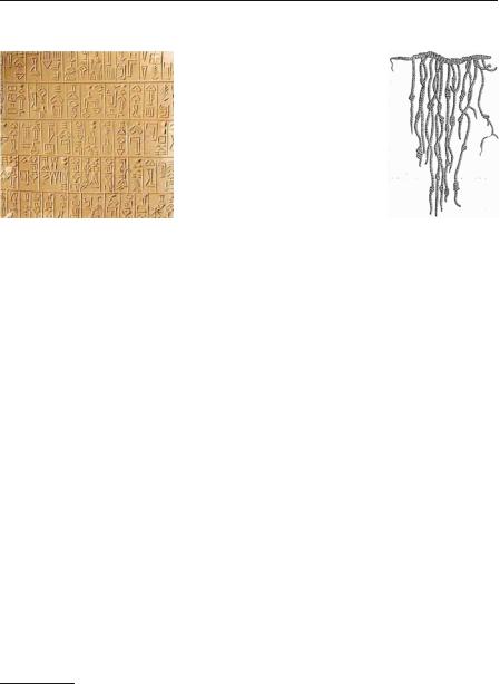
Perhaps the world’s oldest data structures were the tablets in cuneiform script1 used more than 5 000 years ago by custodians in Sumerian temples. These custodians kept lists of goods, and their quantities, owners, and buyers. The picture on the left shows an example. This was possibly the first application of written language. The operations performed on such lists have remained the same – adding entries, storing them for later, searching entries and changing them, going through a list to compile summaries, etc. The Peruvian quipu [137] that you see in the picture on the right served a similar purpose in the Inca empire, using knots in colored strings arranged sequentially on a master string. It is probably easier to maintain and use data on tablets than to use knotted string, but one would not want to haul stone tablets over Andean mountain trails. It is apparent that different representations make sense for the same kind of data.
The abstract notion of a sequence, list, or table is very simple and is independent of its representation in a computer. Mathematically, the only important property is that the elements of a sequence s = e0, . . . , en−1 are arranged in a linear order – in contrast to the trees and graphs discussed in Chaps. 7 and 8, or the unordered hash tables discussed in Chap. 4. There are two basic ways of referring to the elements of a sequence.
One is to specify the index of an element. This is the way we usually think about arrays, where s[i] returns the i-th element of a sequence s. Our pseudocode supports static arrays. In a static data structure, the size is known in advance, and the data structure is not modifiable by insertions and deletions. In a bounded data structure, the maximal size is known in advance. In Sect. 3.2, we introduce dynamic or un-
1The 4 600 year old tablet at the top left is a list of gifts to the high priestess of Adab (see commons.wikimedia.org/wiki/Image:Sumerian_26th_c_Adab.jpg).