Algorithms and data structures

parallel processors than merging-based algorithms. Furthermore, similar algorithms can be used for fast external sorting of integer keys along the lines of Sect. 5.6.

Instead of the single pivot element of quicksort, we now use k − 1 splitter elements s1,. . . , sk−1 to split an input sequence into k output sequences, or buckets. Bucket i gets the elements e for which si−1 ≤ e < si. To simplify matters, we deÞne the artiÞcial splitters s0 = −∞ and sk = ∞ and assume that all elements have different keys. The splitters should be chosen in such a way that the buckets have a size of roughly n/k. The buckets are then sorted recursively. In particular, buckets that Þt into the internal memory can subsequently be sorted internally. Note the similarity to MSD-radix sort described in Sect. 5.6.

The main challenge is to Þnd good splitters quickly. Sample sort uses a fast, simple randomized strategy. For some integer a, we randomly choose (a + 1)k − 1 sample elements from the input. The sample S is then sorted internally, and we deÞne the splitters as si = S[(a+ 1)i] for 1 ≤ i ≤ k −1, i.e., consecutive splitters are separated by a samples, the Þrst splitter is preceded by a samples, and the last splitter is followed by a samples. Taking a = 0 results in a small sample set, but the splitting will not be very good. Moving all elements to the sample will result in perfect splitters, but the sample will be too big. The following analysis shows that setting a = O(log k) achieves roughly equal bucket sizes at low cost for sampling and sorting the sample.

The most I/O-intensive part of sample sort is the k-way distribution of the input sequence to the buckets. We keep one buffer block for the input sequence and one buffer block for each bucket. These buffers are handled analogously to the buffer blocks in k-way merging. If the splitters are kept in a sorted array, we can Þnd the right bucket for an input element e in time O(log k) using binary search.

We leave the detailed proof to the reader and describe only the key ingredient of the analysis here. We use k = Θ(min(n/M, M/B)) buckets and a sample of size O(k log k). The following lemma shows that with this sample size, it is unlikely that any bucket has a size much larger than the average. We hide the constant factors behind O(·) notation because our analysis is not very tight in this respect.

Lemma 5.11. Let k ≥ 2 and a + 1 = 12 ln k. A sample of size (a + 1)k − 1 suffices to ensure that no bucket receives more than 4n/k elements with probability at least 1/2.

Proof. As in our analysis of quicksort (Theorem 5.6), it is useful to study the sorted version s = e1, . . . , en of the input. Assume that there is a bucket with at least 4n/k elements assigned to it. We estimate the probability of this event.

We split s into k/2 segments of length 2n/k. The j-th segment t j contains ele-

ments e2 jn/k+1 to e2( j+1)n/k. If 4n/k elements end up in some bucket, there must be some segment t j such that all its elements end up in the same bucket. This can only

122 5 Sorting and Selection

happen if fewer than a + 1 samples are taken from t j, because otherwise at least one splitter would be chosen from t j and its elements would not end up in a single bucket. Let us concentrate on a Þxed j.

We use a random variable X to denote the number of samples taken from t j. Recall that we take (a + 1)k − 1 samples. For each sample i, 1 ≤ i ≤ (a + 1)k − 1, we deÞne an indicator variable Xi with Xi = 1 if the i-th sample is taken from t j and Xi = 0 otherwise. Then X = ∑1≤i≤(a+1)k−1 Xi. Also, the XiÕs are independent, and prob(Xi = 1) = 2/k. Independence allows us to use the Chernoff bound (A.5) to estimate the probability that X < a + 1. We have

Hence X < a + 1 implies X < (1 −1/3)E[X], and so we can use (A.5) with ε = 1/3. Thus

prob(X < a + 1) ≤ e−(1/9)E[X]/2 ≤ e−(a+1)/12 = e−ln k = 1k .

The probability that an insufÞcient number of samples is chosen from a Þxed t j is thus at most 1/k, and hence the probability that an insufÞcient number is chosen from some t j is at most (k/2) ·(1/k) = 1/2. Thus, with probability at least 1/2, each bucket receives fewer than 4n/k elements.

Exercise 5.32. Work out the details of an external-memory implementation of sample sort. In particular, explain how to implement multiway distribution using 2n/B + k + 1 I/O steps if the internal memory is large enough to store k + 1 blocks of data and O(k) additional elements.

Exercise 5.33 (many equal keys). Explain how to generalize multiway distribution so that it still works if some keys occur very often. Hint: there are at least two different solutions. One uses the sample to Þnd out which elements are frequent. Another solution makes all elements unique by interpreting an element e at an input position i as the pair (e, i).

*Exercise 5.34 (more accurate distribution). A larger sample size improves the quality of the distribution. Prove that a sample of size O (k/ε 2) log(k/ε m) guarantees, with probability (at least 1 − 1/m), that no bucket has more than (1 + ε )n/k elements. Can you get rid of the ε in the logarithmic factor?

5.8 Implementation Notes

Comparison-based sorting algorithms are usually available in standard libraries, and so you may not have to implement one yourself. Many libraries use tuned implementations of quicksort.

Canned non-comparison-based sorting routines are less readily available. Figure 5.15 shows a careful array-based implementation of Ksort. It works well for

Fig. 5.15. Array-based sorting with keys in the range 0..K − 1. The input is an unsorted array a. The output is b, containing the elements of a in sorted order. We Þrst count the number of inputs for each key. Then we form the partial sums of the counts. Finally, we write each input element to the correct position in the output array

small to medium-sized problems. For large K and n, it suffers from the problem that the distribution of elements to the buckets may cause a cache fault for every element.

To Þx this problem, one can use multiphase algorithms similar to MSD radix sort. The number K of output sequences should be chosen in such a way that one block from each bucket is kept in the cache (see also [134]). The distribution degree K can be larger when the subarray to be sorted Þts into the cache. We can then switch to a variant of uniformSort (see Fig. 5.13).

Another important practical aspect concerns the type of elements to be sorted. Sometimes we have rather large elements that are sorted with respect to small keys. For example, you may want to sort an employee database by last name. In this situation, it makes sense to Þrst extract the keys and store them in an array together with pointers to the original elements. Then, only the keyÐpointer pairs are sorted. If the original elements need to be brought into sorted order, they can be permuted accordingly in linear time using the sorted keyÐpointer pairs.

Multiway merging of a small number of sequences (perhaps up to eight) deserves special mention. In this case, the priority queue can be kept in the processor registers [160, 206].

5.8.1 C/C++

Sorting is one of the few algorithms that is part of the C standard library. However, the C sorting routine qsort is slower and harder to use than the C++ function sort. The main reason is that the comparison function is passed as a function pointer and is called for every element comparison. In contrast, sort uses the template mechanism of C++ to Þgure out at compile time how comparisons are performed so that the code generated for comparisons is often a single machine instruction. The parameters passed to sort are an iterator pointing to the start of the sequence to be sorted, and an iterator pointing after the end of the sequence. In our experiments using an Intel Pentium III and GCC 2.95, sort on arrays ran faster than our manual implementation of quicksort. One possible reason is that compiler designers may tune their

124 5 Sorting and Selection

code optimizers until they Þnd that good code for the library version of quicksort is generated. There is an efÞcient parallel-disk external-memory sorter in STXXL [48], an external-memory implementation of the STL. EfÞcient parallel sorters (parallel quicksort and parallel multiway mergesort) for multicore machines are available with the Multi-Core Standard Template Library [180, 125].

Exercise 5.35. Give a C or C++ implementation of the procedure qSort in Fig. 5.7. Use only two parameters: a pointer to the (sub)array to be sorted, and its size.

5.8.2 Java

The Java 6 platform provides a method sort which implements a stable binary mergesort for Arrays and Collections. One can use a customizable Comparator, but there is also a default implementation for all classes supporting the interface Comparable.

5.9 Historical Notes and Further Findings

In later chapters, we shall discuss several generalizations of sorting. Chapter 6 discusses priority queues, a data structure that supports insertions of elements and removal of the smallest element. In particular, inserting n elements followed by repeated deletion of the minimum amounts to sorting. Fast priority queues result in quite good sorting algorithms. A further generalization is the search trees introduced in Chap. 7, a data structure for maintaining a sorted list that allows searching, inserting, and removing elements in logarithmic time.

We have seen several simple, elegant, and efÞcient randomized algorithms in this chapter. An interesting question is whether these algorithms can be replaced by deterministic ones. Blum et al. [25] described a deterministic median selection algorithm that is similar to the randomized algorithm discussed in Sect. 5.5. This deterministic algorithm makes pivot selection more reliable using recursion: it splits the input set into subsets of Þve elements, determines the median of each subset by sorting the Þve-element subset, then determines the median of the n/5 medians by calling the algorithm recursively, and Þnally uses the median of the medians as the splitter. The resulting algorithm has linear worst-case execution time, but the large constant factor makes the algorithm impractical. (We invite the reader to set up a recurrence for the running time and to show that it has a linear solution.)

There are quite practical ways to reduce the expected number of comparisons required by quicksort. Using the median of three random elements yields an algorithm with about 1.188n logn comparisons. The median of three medians of three-element subsets brings this down to ≈ 1.094n logn [20]. The number of comparisons can be reduced further by making the number of elements considered for pivot selection de-

pendent on the size of the subproblem. Martinez and Roura [123] showed that for a

√

subproblem of size m, the median of Θ( m) elements is a good choice for the pivot. With this approach, the total number of comparisons becomes (1 + o(1))n log n, i.e., it matches the lower bound of n log n − O(n) up to lower-order terms. Interestingly,

the above optimizations can be counterproductive. Although fewer instructions are executed, it becomes impossible to predict when the inner while loops of quicksort will be aborted. Since modern, deeply pipelined processors only work efÞciently when they can predict the directions of branches taken, the net effect on performance can even be negative [102]. Therefore, in [167] , a comparison-based sorting algorithm that avoids conditional branch instructions was developed. An interesting deterministic variant of quicksort is proportion-extend sort [38].

A classical sorting algorithm of some historical interest is Shell sort [174, 100], a generalization of insertion sort, that gains efÞciency by also comparing nonadjacent elements. It is still open whether some variant of Shell sort achieves O(n log n) average running time [100, 124].

There are some interesting techniques for improving external multiway mergesort. The snow plow heuristic [112, Sect. 5.4.1] forms runs of expected size 2M using a fast memory of size M: whenever an element is selected from the internal priority queue and written to the output buffer and the next element in the input buffer can extend the current run, we add it to the priority queue. Also, the use of tournament trees instead of general priority queues leads to a further improvement of multiway merging [112].

Parallelism can be used to improve the sorting of very large data sets, either in the form of a uniprocessor using parallel disks or in the form of a multiprocessor. Multiway mergesort and distribution sort can be adapted to D parallel disks by striping, i.e., any D consecutive blocks in a run or bucket are evenly distributed over the disks. Using randomization, this idea can be developed into almost optimal algorithms that also overlap I/O and computation [49]. The sample sort algorithm of Sect. 5.7.2 can be adapted to parallel machines [24] and results in an efÞcient parallel sorter.

We have seen linear-time algorithms for highly structured inputs. A quite general model, for which the n log n lower bound does not hold, is the word model. In this model, keys are integers that Þt into a single memory cell, say 32or 64-bit keys, and the standard operations on words (bitwise-AND, bitwise-OR, addition, . . . ) are

available in constant time. In this model, sorting is possible in deterministic time

√

O(n log log n) [11]. With randomization, even O n log log n is possible [85]. Flash sort [149] is a distribution-based algorithm that works almost in-place.

Exercise 5.36 (Unix spellchecking). Assume you have a dictionary consisting of a sorted sequence of correctly spelled words. To check a text, you convert it to a sequence of words, sort it, scan the text and dictionary simultaneously, and output the words in the text that do not appear in the dictionary. Implement this spellchecker using Unix tools in a small number of lines of code. Can you do this in one line?

6

Priority Queues

The company TMG markets tailor-made first-rate garments. It organizes marketing, measurements, etc., but outsources the actual fabrication to independent tailors. The company keeps 20% of the revenue. When the company was founded in the 19th century, there were five subcontractors. Now it controls 15% of the world market and there are thousands of subcontractors worldwide.

Your task is to assign orders to the subcontractors. The rule is that an order is assigned to the tailor who has so far (in the current year) been assigned the smallest total value of orders. Your ancestors used a blackboard to keep track of the current total value of orders for each tailor; in computer science terms, they kept a list of values and spent linear time to find the correct tailor. The business has outgrown this solution. Can you come up with a more scalable solution where you have to look only at a small number of values to decide who will be assigned the next order?

In the following year the rules are changed. In order to encourage timely delivery, the orders are now assigned to the tailor with the smallest value of unfinished orders, i.e., whenever a finished order arrives, you have to deduct the value of the order from the backlog of the tailor who executed it. Is your strategy for assigning orders flexible enough to handle this efficiently?

Priority queues are the data structure required for the problem above and for many other applications. We start our discussion with the precise specification. Priority queues maintain a set M of Elements with Keys under the following operations:

This is enough for the first part of our example. Each year, we build a new priority queue containing an Element with a Key of zero for each contract tailor. To assign an order, we delete the smallest Element, add the order value to its Key, and reinsert it. Section 6.1 presents a simple, efficient implementation of this basic functionality.

0The photograph shows a queue at the Mao Mausoleum (V. Berger, see http://commons.wikimedia.org/wiki/Image:Zhengyangmen01.jpg).

128 6 Priority Queues

Addressable priority queues additionally support operations on arbitrary elements addressed by an element handle h:

•insert: as before, but return a handle to the element inserted.

•remove(h): remove the element specified by the handle h.

•decreaseKey(h, k): decrease the key of the element specified by the handle h to k.

In our example, the operation remove might be helpful when a contractor is fired because he/she delivers poor quality. Using this operation together with insert, we can also implement the “new contract rules”: when an order is delivered, we remove the Element for the contractor who executed the order, subtract the value of the order from its Key value, and reinsert the Element. DecreaseKey streamlines this process to a single operation. In Sect. 6.2, we shall see that this is not just convenient but that decreasing keys can be implemented more efficiently than arbitrary element updates.

Priority queues have many applications. For example, in Sect. 12.2, we shall see that our introductory example can also be viewed as a greedy algorithm for a machine-scheduling problem. Also, the rather naive selection-sort algorithm of Sect. 5.1 can be implemented efficiently now: first, insert all elements into a priority queue, and then repeatedly delete the smallest element and output it. A tuned version of this idea is described in Sect. 6.1. The resulting heapsort algorithm is popular because it needs no additional space and is worst-case efficient.

In a discrete-event simulation, one has to maintain a set of pending events. Each event happens at some scheduled point in time and creates zero or more new events in the future. Pending events are kept in a priority queue. The main loop of the simulation deletes the next event from the queue, executes it, and inserts newly generated events into the priority queue. Note that the priorities (times) of the deleted elements (simulated events) increase monotonically during the simulation. It turns out that many applications of priority queues have this monotonicity property. Section 10.5 explains how to exploit monotonicity for integer keys.

Another application of monotone priority queues is the best-first branch-and- bound approach to optimization described in Sect. 12.4. Here, the elements are partial solutions of an optimization problem and the keys are optimistic estimates of the obtainable solution quality. The algorithm repeatedly removes the best-looking partial solution, refines it, and inserts zero or more new partial solutions.

We shall see two applications of addressable priority queues in the chapters on graph algorithms. In both applications, the priority queue stores nodes of a graph. Dijkstra’s algorithm for computing shortest paths (Sect. 10.3) uses a monotone priority queue where the keys are path lengths. The Jarník–Prim algorithm for computing minimum spanning trees (Sect. 11.2) uses a (nonmonotone) priority queue where the keys are the weights of edges connecting a node to a partial spanning tree. In both algorithms, there can be a decreaseKey operation for each edge, whereas there is at most one insert and deleteMin for each node. Observe that the number of edges may be much larger than the number of nodes, and hence the implementation of decreaseKey deserves special attention.

Exercise 6.1. Show how to implement bounded nonaddressable priority queues using arrays. The maximal size of the queue is w and when the queue has a size n, the first n entries of the array are used. Compare the complexity of the queue operations for two implementations: one by unsorted arrays and one by sorted arrays.

Exercise 6.2. Show how to implement addressable priority queues using doubly linked lists. Each list item represents an element in the queue, and a handle is a handle of a list item. Compare the complexity of the queue operations for two implementations: one by sorted lists and one by unsorted lists.

6.1 Binary Heaps

Heaps are a simple and efficient implementation of nonaddressable bounded priority queues [208]. They can be made unbounded in the same way as bounded arrays can be made unbounded (see Sect. 3.2). Heaps can also be made addressable, but we shall see better addressable queues in later sections.

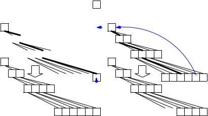
Fig. 6.1. The top part shows a heap with n = 12 elements stored in an array h with w = 13 entries. The root corresponds to index 1. The children of the root correspond to indices 2 and 3. The children of node i have indices 2i and 2i + 1 (if they exist). The parent of a node i, i ≥ 2, has index i/2 . The elements stored in this implicitly defined tree fulfill the invariant that parents are no larger than their children, i.e., the tree is heap-ordered. The left part shows the effect of inserting b. The thick edges mark a path from the rightmost leaf to the root. The new element b is moved up this path until its parent is smaller. The remaining elements on the path are moved down to make room for b. The right part shows the effect of deleting the minimum. The thick edges mark the path p that starts at the root and always proceeds to the child with the smaller Key. The element q is provisionally moved to the root and then moves down p until its successors are larger. The remaining elements move up to make room for q

Fig. 6.2. A class for a priority queue based on binary heaps whose size is bounded by w

We use an array h[1..w] that stores the elements of the queue. The first n entries of the array are used. The array is heap-ordered, i.e.,

for j with 2 ≤ j ≤ n: h[ j/2 ] ≤ h[ j ].

What does "heap-ordered" mean? The key to understanding this definition is a bijection between positive integers and the nodes of a complete binary tree, as illustrated in Fig. 6.1. In a heap the minimum element is stored in the root (= array position 1). Thus min takes time O(1). Creating an empty heap with space for w elements also takes constant time, as it only needs to allocate an array of size w. Figure 6.2 gives pseudocode for this basic setup.

The minimum of a heap is stored in h[1] and hence can be found in constant time; this is the same as for a sorted array. However, the heap property is much less restrictive than the property of being sorted. For example, there is only one sorted version of the set {1, 2, 3}, but both 1, 2, 3 and 1, 3, 2 are legal heap representations.

Exercise 6.3. Give all representations of {1, 2, 3, 4} as a heap.

We shall next see that the increased flexibility permits efficient implementations of insert and deleteMin. We choose a description which is simple and can be easily proven correct. Section 6.4 gives some hints toward a more efficient implementation. An insert puts a new element e tentatively at the end of the heap h, i.e., into h[n], and then moves e to an appropriate position on the path from leaf h[n] to the root:

Procedure insert(e : Element) assert n < w

n++; h[n] := e siftUp(n)

Here siftUp(s) moves the contents of node s toward the root until the heap property holds (see. Fig. 6.1).

Procedure siftUp(i : N)

assert the heap property holds except maybe at position i if i = 1 h[ i/2 ] ≤ h[i] then return

assert the heap property holds except for position i swap(h[i], h[ i/2 ])

assert the heap property holds except maybe for position i/2 siftUp( i/2 )

Correctness follows from the invariants stated.

Exercise 6.4. Show that the running time of siftUp(n) is O(log n) and hence an insert takes time O(log n).

A deleteMin returns the contents of the root and replaces them by the contents of node n. Since h[n] might be larger than h[2] or h[3], this manipulation may violate the heap property at position 2 or 3. This possible violation is repaired using siftDown:

Function deleteMin : Element assert n > 0

result = h[1] : Element h[1] := h[n]; n-- siftDown(1)

return result

The procedure siftDown(1) moves the new contents of the root down the tree until the heap property holds. More precisely, consider the path p that starts at the root and always proceeds to the child with the smaller key (see Fig. 6.1); in the case of equal keys, the choice is arbitrary. We extend the path until all children (there may be zero, one, or two) have a key no larger than h[1]. We put h[1] into this position and move all elements on path p up by one position. In this way, the heap property is restored. This strategy is most easily formulated as a recursive procedure. A call of the following procedure siftDown(i) repairs the heap property in the subtree rooted at i, assuming that it holds already for the subtrees rooted at 2i and 2i + 1; the heap property holds in the subtree rooted at i if we have h[ j/2 ] ≤ h[ j] for all proper descendants j of i:

Procedure siftDown(i : N)

assert the heap property holds for the trees rooted at j = 2i and j = 2i + 1 if 2i ≤ n then // i is not a leaf

if 2i + 1 > n h[2i] ≤ h[2i + 1] then m := 2i else m := 2i + 1 assert the sibling of m does not exist or it has a larger key than m

assert the heap property holds for the tree rooted at i

Exercise 6.5. Our current implementation of siftDown needs about 2 log n element comparisons. Show how to reduce this to log n + O(log log n). Hint: determine the path p first and then perform a binary search on this path to find the proper position for h[1]. Section 6.5 has more on variants of siftDown.

We can obviously build a heap from n elements by inserting them one after the other in O(n log n) total time. Interestingly, we can do better by establishing the heap property in a bottom-up fashion: siftDown allows us to establish the heap property for a subtree of height k + 1 provided the heap property holds for its subtrees of height k. The following exercise asks you to work out the details of this idea.