Algorithms and data structures

The basic dynamic-programming algorithm for the knapsack problem and also its optimization require Θ (nM) worst-case time. This is quite good if M is not too large. Since the running time is polynomial in n and M, the algorithm is called pseudopolynomial. The ÒpseudoÓ means that it is not necessarily polynomial in the input size measured in bits; however, it is polynomial in the natural parameters n and M. There is, however, an important difference between the basic and the reÞned approach. The basic approach has best-case running time Θ (nM). The best case for the reÞned approach is O(n). The average-case complexity of the reÞned algorithm is polynomial in n, independent of M. This holds even if the averaging is done only over perturbations of an arbitrary instance by a small amount of random noise. We refer the reader to [17] for details.

Exercise 12.13 (dynamic programming by profit). DeÞne W (i, P) to be the smallest weight needed to achieve a proÞt of at least P using knapsack items 1..i.

(a)Show that W (i, P) = min {W (i − 1, P),W (i − 1, P − pi) + wi}.

(b)Develop a table-based dynamic-programming algorithm using the above recurrence that computes optimal solutions to the knapsack problem in time O(np ), where p is the proÞt of the optimal solution. Hint: assume Þrst that p , or at least a good upper bound for it, is known. Then remove this assumption.

Exercise 12.14 (making change). Suppose you have to program a vending machine that should give exact change using a minimum number of coins.

(a)Develop an optimal greedy algorithm that works in the euro zone with coins worth 1, 2, 5, 10, 20, 50, 100, and 200 cents and in the dollar zone with coins worth 1, 5, 10, 25, 50, and 100 cents.

(b)Show that this algorithm would not be optimal if there were also a 4 cent coin.

(c)Develop a dynamic-programming algorithm that gives optimal change for any currency system.

Exercise 12.15 (chained matrix products). We want to compute the matrix product

M1M2 ···Mn, where Mi is a ki−1 × ki matrix. Assume that a pairwise matrix product is computed in the straightforward way using mks element multiplications to obtain the product of an m × k matrix with a k × s matrix. Exploit the associativity of matrix products to minimize the number of element multiplications needed. Use dynamic programming to Þnd an optimal evaluation order in time O n3 . For example, the product of a 4 × 5 matrix M1, a 5 × 2 matrix M2, and a 2 × 8 matrix M3 can be computed in two ways. Computing M1(M2M3) takes 5 · 2 · 8 + 4 · 5 · 8 = 240 multiplications, whereas computing (M1M2)M3 takes only 4 · 5 · 2 + 4 · 2 · 8 = 104 multiplications.

Exercise 12.16 (minimum edit distance). The minimum edit distance (or Levenshtein distance) L(s, t) between two strings s and t is the minimum number of character deletions, insertions, and replacements applied to s that produces the string t. For example, L(graph, group) = 3 (delete h, replace a by o, insert u before p). DeÞne d(i, j) = L( s1, . . . , si , t1, . . . , t j ). Show that

246 12 Generic Approaches to Optimization

d(i, j) = min d(i − 1, j) + 1, d(i, j − 1) + 1, d(i − 1, j − 1) + [si =t j]

where [si =t j] is one if si and t j are different and is zero otherwise.

Exercise 12.17. Does the principle of optimality hold for minimum spanning trees? Check the following three possibilities for deÞnitions of subproblems: subsets of nodes, arbitrary subsets of edges, and preÞxes of the sorted sequence of edges.

Exercise 12.18 (constrained shortest path). Consider a directed graph G = (V, E) where edges e E have a length (e) and a cost c(e). We want to Þnd a path from node s to node t that minimizes the total length subject to the constraint that the total cost of the path is at most C. Show that subpaths s , t of optimal solutions are not necessarily shortest paths from s to t .

12.4 Systematic Search – When in Doubt, Use Brute Force

In many optimization problems, the universe U of possible solutions is Þnite, so that we can in principle solve the optimization problem by trying all possibilities. Naive application of this idea does not lead very far, however, but we can frequently restrict the search to promising candidates, and then the concept carries a lot further.

We shall explain the concept of systematic search using the knapsack problem and a speciÞc approach to systematic search known as branch-and-bound. In Exercises 12.20 and 12.21, we outline systematic-search routines following a somewhat different pattern.

Figure 12.5 gives pseudocode for a systematic-search routine bbKnapsack for the knapsack problem and Figure 12.6 shows a sample run. Branching is the most fundamental ingredient of systematic-search routines. All sensible values for some piece of the solution are tried. For each of these values, the resulting problem is solved recursively. Within the recursive call, the chosen value is Þxed. The routine bbKnapsack Þrst tries including an item by setting xi := 1, and then excluding it by setting xi := 0. The variables are Þxed one after another in order of decreasing proÞt density. The assignment xi := 1 is not tried if this would exceed the remaining knapsack capacity M . With these deÞnitions, after all variables have been set, in the n-th level of recursion, bbKnapsack will have found a feasible solution. Indeed, without the bounding rule below, the algorithm would systematically explore all possible solutions and the first feasible solution encountered would be the solution found by the algorithm greedy. The (partial) solutions explored by the algorithm form a tree. Branching happens at internal nodes of this tree.

Bounding is a method for pruning subtrees that cannot contain optimal solutions. A branch-and-bound algorithm keeps the best feasible solution found in a global variable xö; this solution is often called the incumbent solution. It is initialized to a solution determined by a heuristic routine and, at all times, provides a lower bound p · xö on the value of the objective function that can be obtained. This lower bound is complemented by an upper bound u for the value of the objective function obtainable by extending the current partial solution x to a full feasible solution. In our example,

// Find solutions assuming x1, . . . , xi−1 are Þxed, M = M − ∑ xiwi, P = ∑ xi pi.

if wi ≤ M then xi := 1; recurse(i + 1, M − wi, P + pi) if u > p · xö then xi := 0; recurse(i + 1, M , P)

Fig. 12.5. A branch-and-bound algorithm for the knapsack problem. An initial feasible solution is constructed by the function heuristicKnapsack using some heuristic algorithm. The function upperBound computes an upper bound for the possible proÞt

C improved solution

Fig. 12.6. The search space explored by knapsackBB for a knapsack instance with p = (10, 20, 15, 20), w = (1, 3, 2, 4), and M = 5, and an empty initial solution xö = (0, 0, 0, 0). The function upperBound is computed by rounding down the optimal value of the objective function for the fractional knapsack problem. The nodes of the search tree contain x1 ···xi−1 and the upper bound u. Left children are explored Þrst and correspond to setting xi := 1. There are two reasons for not exploring a child: either there is not enough capacity left to include an element (indicated by C), or a feasible solution with a proÞt equal to the upper bound is already known (indicated by B)

the upper bound could be the proÞt for the fractional knapsack problem with items

i..n and capacity M = M − ∑ j<i xiwi.

Branch-and-bound stops expanding the current branch of the search tree when u ≤ p · xö, i.e., when there is no hope of an improved solution in the current subtree of the search space. We test u > p · xö again before exploring the case xi = 0 because xö might change when the case xi = 1 is explored.

248 12 Generic Approaches to Optimization

Exercise 12.19. Explain how to implement the function upperBound in Fig. 12.5 so that it runs in time O(log n). Hint: precompute the preÞx sums ∑k≤i wi and ∑k≤i pi and use binary search.

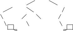
Exercise 12.20 (the 15-puzzle). The 15-puzzle is a popular sliding-block puzzle. You have to move 15 square tiles in a 4 ×4 frame into the right order. DeÞne a move as the action of interchanging a square and the hole in the array of tiles.

Design an algorithm that Þnds a shortest-move sequence from a given starting conÞguration to the ordered conÞguration shown at the bottom of the Þgure on the left. Use iterative deepening depth-first search [114]: try all one-move sequences Þrst, then all two-move sequences, and so on. This should work for the simpler 8-puzzle. For the 15-puzzle, use the following optimizations. Never undo the immediately preceding move. Use the number of moves that would be needed if all pieces could be moved freely as a lower bound and stop exploring a subtree if this bound proves that the current search depth is too small. Decide beforehand whether the number of moves is odd or even. Implement your algorithm to run in constant time per move tried.

Exercise 12.21 (constraint programming and the eight-queens problem). Consider a chessboard. The task is to place eight queens on the board so that they do not attack each other, i.e., no two queens should be placed in the same row, column, diagonal, or antidiagonal. So each row contains exactly one queen. Let xi be the position of the queen in row i. Then xi 1..8. The solution must satisfy the following constraints: xi =x j, i + xi =j + x j, and xi − i =x j − j for 1 ≤ i < j ≤ 8. What do these conditions express? Show that they are sufÞcient. A systematic search can use the following optimization. When a variable xi is Þxed at some value, this excludes some values for variables that are still free. Modify the systematic search so that it keeps track of the values that are still available for free variables. Stop exploration as soon as there is a free variable that has no value available to it anymore. This technique of eliminating values is basic to constraint programming.

12.4.1 Solving Integer Linear Programs

In Sect. 12.1.1, we have seen how to formulate the knapsack problem as a 0 Ð1 integer linear program. We shall now indicate how the branch-and-bound procedure developed for the knapsack problem can be applied to any 0 Ð1 integer linear program. Recall that in a 0 Ð1 integer linear program the values of the variables are constrained to 0 and 1. Our discussion will be brief, and we refer the reader to a textbook on integer linear programming [147, 172] for more information.

The main change is that the function upperBound now solves a general linear program that has variables xi,. . . ,xn with range [0, 1]. The constraints for this LP

come from the input ILP, with the variables x1 to xi−1 replaced by their values. In the remainder of this section, we shall simply refer to this linear program as Òthe LPÓ.

If the LP has a feasible solution, upperBound returns the optimal value for the LP. If the LP has no feasible solution, upperBound returns −∞ so that the ILP solver will stop exploring this branch of the search space. We shall describe next several generalizations of the basic branch-and-bound procedure that sometimes lead to considerable improvements.

Branch Selection: We may pick any unÞxed variable x j for branching. In particular, we can make the choice depend on the solution of the LP. A commonly used rule is to branch on a variable whose fractional value in the LP is closest to 1/2.

Order of Search Tree Traversal: In the knapsack example, the search tree was traversed depth-Þrst, and the 1-branch was tried Þrst. In general, we are free to choose any order of tree traversal. There are at least two considerations inßuencing the choice of strategy. If no good feasible solution is known, it is good to use a depth-Þrst strategy so that complete solutions are explored quickly. Otherwise, it is better to use a best-first strategy that explores those search tree nodes that are most likely to contain good solutions. Search tree nodes are kept in a priority queue, and the next node to be explored is the most promising node in the queue. The priority could be the upper bound returned by the LP. However, since the LP is expensive to evaluate, one sometimes settles for an approximation.

Finding Solutions: We may be lucky in that the solution of the LP turns out to assign integer values to all variables. In this case there is no need for further branching. Application-speciÞc heuristics can additionally help to Þnd good solutions quickly.

Branch-and-Cut: When an ILP solver branches too often, the size of the search tree explodes and it becomes too expensive to Þnd an optimal solution. One way to avoid branching is to add constraints to the linear program that cut away solutions with fractional values for the variables without changing the solutions with integer values.

12.5 Local Search – Think Globally, Act Locally

The optimization algorithms we have seen so far are applicable only in special circumstances. Dynamic programming needs a special structure of the problem and may require a lot of space and time. Systematic search is usually too slow for large inputs. Greedy algorithms are fast but often yield only low-quality solutions. Local search is a widely applicable iterative procedure. It starts with some feasible solution and then moves from feasible solution to feasible solution by local modiÞcations. Figure 12.7 gives the basic framework. We shall reÞne it later.

Local search maintains a current feasible solution x and the best solution xö seen so far. In each step, local search moves from the current solution to a neighboring solution. What are neighboring solutions? Any solution that can be obtained from the current solution by making small changes to it. For example, in the case of the

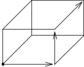
half-space. Hyperplanes are the n-dimensional analogues of planes and half-spaces are the analogues of half-planes. The set of feasible solutions is an intersection of m half-spaces and hyperplanes and forms a convex polytope. We have already seen an example in two-dimensional space in Fig. 12.2. Figure 12.8 shows an example in three-dimensional space. Convex polytopes are the n-dimensional analogues of convex polygons. In the interior of the polytope, all inequalities are strict (= satisÞed with inequality); on the boundary some inequalities are tight (= satisÞed with equality). The vertices and edges of the polytope are particularly important parts of the boundary. We shall now sketch how the simplex algorithm works. We assume that there are no equality constraints. Observe that an equality constraint c can be solved for any one of its variables; this variable can then be removed by substituting into the other equalities and inequalities. Afterwards, the constraint c is redundant and can be dropped.

The simplex algorithm starts at an arbitrary vertex of the feasible region. In each step, it moves to a neighboring vertex, i.e., a vertex reachable via an edge, with a larger objective value. If there is more than one such neighbor, a common strategy is to move to the neighbor with the largest objective value. If there is no neighbor with a larger objective value, the algorithm stops. At this point, the algorithm has found the vertex with the maximal objective value. In the examples in Figs. 12.2 and 12.8, the captions argue why this is true. The general argument is as follows. Let x be the vertex at which the simplex algorithm stops. The feasible region is contained in a cone with apex x and spanned by the edges incident on x . All these edges go to vertices with smaller objective values and hence the entire cone is contained in the half-space {x : c · x ≤ c · x }. Thus no feasible point can have an objective value

(1,1,1)

(1,0,1)

Fig. 12.8. The three-dimensional unit cube is deÞned by the inequalities x ≥ 0, x ≤ 1, y ≥ 0, y ≤ 1, z ≥ 0, and z ≤ 1. At the vertices (1, 1, 1) and (1, 0, 1), three inequalities are tight, and on the edge connecting these vertices, the inequalities x ≤ 1 and z ≤ 1 are tight. For the objective Òmaximize x + y + zÓ, the simplex algorithm starting at (0, 0, 0) may move along the path indicated by arrows. The vertex (1, 1, 1) is optimal, since the half-space x + y + z ≤ 3 contains the entire feasible region and has (1, 1, 1) in its boundary

252 12 Generic Approaches to Optimization

larger than x . We have described the simplex algorithm as a walk on the boundary of a convex polytope, i.e., in geometric language. It can be described equivalently using the language of linear algebra. Actual implementations use the linear-algebra description.

In the case of linear programming, hill climbing leads to an optimal solution. In general, however, hill climbing will not Þnd an optimal solution. In fact, it will not even Þnd a near-optimal solution. Consider the following example. Our task is to Þnd the highest point on earth, i.e., Mount Everest. A feasible solution is any point on earth. The local neighborhood of a point is any point within a distance of 10 km. So the algorithm would start at some point on earth, then go to the highest point within a distance of 10 km, then go again to the highest point within a distance of 10 km, and so on. If one were to start from the Þrst authorÕs home (altitude 206 meters), the Þrst step would lead to an altitude of 350 m, and there the algorithm would stop, because there is no higher hill within 10 km of that point. There are very few places in the world where the algorithm would continue for long, and even fewer places where it would Þnd Mount Everest.

Why does hill climbing work so nicely for linear programming, but fail to Þnd Mount Everest? The reason is that the earth has many local optima, hills that are the highest point within a range of 10 km. In contrast, a linear program has only one local optimum (which then, of course, is also a global optimum). For a problem with many local optima, we should expect any generic method to have difÞculties. Observe that increasing the size of the neighborhoods in the search for Mount Everest does not really solve the problem, except if the neighborhoods are made to cover the entire earth. But Þnding the optimum in a neighborhood is then as hard as the full problem.

12.5.2 Simulated Annealing – Learning from Nature

If we want to ban the bane of local optima in local search, we must Þnd a way to escape from them. This means that we sometimes have to accept moves that decrease the objective value. What could ÒsometimesÓ mean in this context? We have contradictory goals. On the one hand, we must be willing to make many downhill steps so that we can escape from wide local optima. On the other hand, we must be sufÞciently target-oriented so that we Þnd a global optimum at the end of a long narrow ridge. A very popular and successful approach for reconciling these contradictory goals is simulated annealing; see Fig. 12.9. This works in phases that are controlled by a parameter T , called the temperature of the process. We shall explain below why the language of physics is used in the description of simulated annealing. In each phase, a number of moves are made. In each move, a neighbor x N (x) ∩ L is chosen uniformly at random, and the move from x to x is made with a certain probability. This probability is one if x improves upon x. It is less than one if the move is to an inferior solution. The trick is to make the probability depend on T . If T is large, we make the move to an inferior solution relatively likely; if T is close to zero, we make such a move relatively unlikely. The hope is that, in this way, the process zeros in on a region containing a good local optimum in phases of high temperature and then actually Þnds a near-optimal solution in the phases of low temperature.

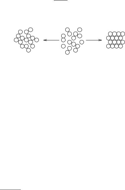
Fig. 12.10. Annealing versus shock cooling

The exact choice of the transition probability in the case where x is an inferior solution is given by exp(( f (x ) − f (x))/T ). Observe that T is in the denominator and that f (x ) − f (x) is negative. So the probability decreases with T and also with the absolute loss in objective value.

Why is the language of physics used, and why this apparently strange choice of transition probabilities? Simulated annealing is inspired by the physical process of annealing, which can be used to minimize6 the global energy of a physical system. For example, consider a pot of molten silica (SiO2); see Fig. 12.10. If we cool it very quickly, we obtain a glass Ð an amorphous substance in which every molecule is in a local minimum of energy. This process of shock cooling has a certain similarity to hill climbing. Every molecule simply drops into a state of locally minimal energy; in hill climbing, we accept a local modiÞcation of the state if it leads to a smaller value of the objective function. However, a glass is not a state of global minimum energy. A state of much lower energy is reached by a quartz crystal, in which all molecules are arranged in a regular way. This state can be reached (or approximated) by cooling the melt very slowly. This process is called annealing. How can it be that molecules arrange themselves into a perfect shape over a distance of billions of molecular diameters although they feel only local forces extending over a few molecular diameters?

Qualitatively, the explanation is that local energy minima have enough time to dissolve in favor of globally more efÞcient structures. For example, assume that a cluster of a dozen molecules approaches a small perfect crystal that already consists of thousands of molecules. Then, with enough time, the cluster will dissolve and

6 Note that we are talking about minimization now.

254 12 Generic Approaches to Optimization

its molecules can attach to the crystal. Here is a more formal description of this process, which can be shown to hold for a reasonable model of the system: if cooling is sufÞciently slow, the system reaches thermal equilibrium at every temperature. Equilibrium at temperature T means that a state x of the system with energy Ex is assumed with probability

exp(−Ex/T )

∑y L exp(−Ey/T )

where T is the temperature of the system and L is the set of states of the system. This energy distribution is called the Boltzmann distribution. When T decreases, the probability of states with a minimal energy grows. Actually, in the limit T → 0, the probability of states with a minimal energy approaches one.

The same mathematics works for abstract systems corresponding to a maximization problem. We identify the cost function f with the energy of the system, and a feasible solution with the state of the system. It can be shown that the system approaches a Boltzmann distribution for a quite general class of neighborhoods and the following rules for choosing the next state:

pick x from N (x) ∩ L uniformly at random

with probability min(1, exp(( f (x ) − f (x))/T )) do x := x .

The physical analogy gives some idea of why simulated annealing might work,7 but it does not provide an implementable algorithm. We have to get rid of two inÞnities: for every temperature, we wait inÞnitely long to reach equilibrium, and do that for inÞnitely many temperatures. Simulated-annealing algorithms therefore have to decide on a cooling schedule, i.e., how the temperature T should be varied over time. A simple schedule chooses a starting temperature T0 that is supposed to be just large enough so that all neighbors are accepted. Furthermore, for a given problem instance, there is a Þxed number N of iterations to be used at each temperature. The idea is that N should be as small as possible but still allow the system to get close to equilibrium. After every N iterations, T is decreased by multiplying it by a constant α less than one. Typically, α is between 0.8 and 0.99. When T has become so small that moves to inferior solutions have become highly unlikely (this is the case when T is comparable to the smallest difference in objective value between any two feasible solutions), T is Þnally set to 0, i.e., the annealing process concludes with a hill-climbing search.

Better performance can be obtained with dynamic schedules. For example, the initial temperature can be determined by starting with a low temperature and increasing it quickly until the fraction of transitions accepted approaches one. Dynamic schedules base their decision about how much T should be lowered on the actually observed variation in f (x) during the local search. If the temperature change is tiny compared with the variation, it has too little effect. If the change is too close to or even larger than the variation observed, there is a danger that the system will be prematurely forced into a local optimum. The number of steps to be made until the temperature is lowered can be made dependent on the actual number of moves

7 Note that we have written Òmight workÓ and not ÒworksÓ.