

Algorithms and data structures
.pdf12.1 Linear Programming Ð a Black-Box Solver |
235 |
kinds of speciÞcation are general solvers available? Here, we introduce a particularly large class of problems for which efÞcient black-box solvers are available.
Definition 12.1. A linear program (LP)2 with n variables and m constraints is a maximization problem defined on a vector x = (x1, . . . , xn) of real-valued variables. The objective function is a linear function f of x, i.e., f : Rn → R with f (x) = c ·x, where c = (c1, . . . , cn) is called cost or proÞt3 vector. The variables are constrained by m linear constraints of the form ai · x i bi, where i {≤, ≥, =}, ai = (ai1, . . . , ain) Rn, and bi R for i 1..m. The set of feasible solutions is given by
L = x Rn : i 1..m and j 1..n : x j ≥ 0 ai · x i bi . |
|
y |
feasible solutions |
|
y ≤ 6 |
|
(2,6) |
|
x + y ≤ 8 |
|
2x − y ≤ 8 |
|
x + 4y ≤ 26 |
|
better |
|
solutions |
|
x |
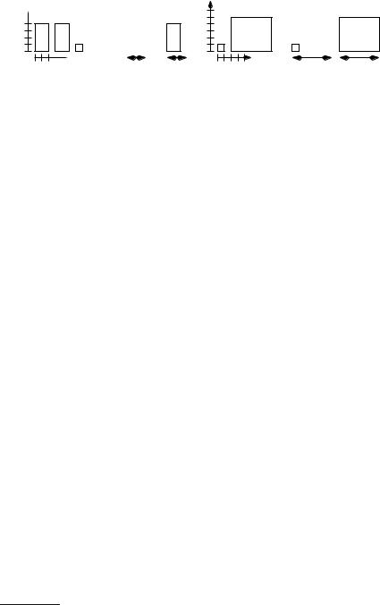
Fig. 12.2. A simple two-dimensional linear program in variables x and y, with three constraints and the objective Òmaximize x + 4yÓ. The feasible region is shaded, and (x, y) = (2, 6) is the optimal solution. Its objective value is 26. The vertex (2, 6) is optimal because the half-plane x + 4y ≤ 26 contains the entire feasible region and has (2, 6) in its boundary
Figure 12.2 shows a simple example. A classical application of linear programming is the diet problem. A farmer wants to mix food for his cows. There are n different kinds of food on the market, say, corn, soya, Þsh meal, . . . . One kilogram of a food j costs c j euros. There are m requirements for healthy nutrition; for example the cows should get enough calories, protein, vitamin C, and so on. One kilogram of food j contains ai j percent of a cowÕs daily requirement with respect to requirement i. A solution to the following linear program gives a cost-optimal diet that satisÞes the health constraints. Let x j denote the amount (in kilogram) of food j used by the
2The term Òlinear programÓ stems from the 1940s [45] and has nothing to do with the modern meaning of ÒprogramÓ as in Òcomputer programÓ.
3It is common to use the term ÒproÞtÓ in maximization problems and ÒcostÓ in minimization problems.
236 12 Generic Approaches to Optimization
farmer. The i-th nutritional requirement is modeled by the inequality ∑ j ai jx j ≥ 100. The cost of the diet is given by ∑ j c jx j. The goal is to minimize the cost of the diet.
Exercise 12.1. How do you model supplies that are available only in limited amounts, for example food produced by the farmer himself? Also, explain how to specify additional constraints such as Òno more than 0.01mg cadmium contamination per cow per dayÓ.
Can the knapsack problem be formulated as a linear program? Probably not. Each item either goes into the knapsack or it does not. There is no possibility of adding an item partially. In contrast, it is assumed in the diet problem that any arbitrary amount of any food can be purchased, for example 3.7245 kg and not just 3 kg or 4 kg. Integer linear programs (see Sect. 12.1.1) are the right tool for the knapsack problem.
We next connect linear programming to the problems that we have studied in previous chapters of the book. We shall show how to formulate the single-source shortest-path problem with nonnegative edge weights as a linear program. Let G = (V, E) be a directed graph, let s V be the source node, and let c : E → R≥0 be the cost function on the edges of G. In our linear program, we have a variable dv for every vertex of the graph. The intention is that dv denotes the cost of the shortest path from s to v. Consider
maximize |
∑dv |
|
v V |
subject to |
ds = 0 |
|
dw ≤ dv + c(e) for all e = (v, w) E . |
Theorem 12.2. Let G = (V, E) be a directed graph, s V a designated vertex, and c : E → R≥0 a nonnegative cost function. If all vertices of G are reachable from s, the shortest-path distances in G are the unique optimal solution to the linear program above.
Proof. Let μ (v) be the length of the shortest path from s to v. Then μ (v) R≥0, since all nodes are reachable from s, and hence no vertex can have a distance +∞ from s. We observe Þrst that dv := μ (v) for all v satisÞes the constraints of the LP. Indeed, μ (s) = 0 and μ (w) ≤ μ (v) + c(e) for any edge e = (v, w).
We next show that if (dv)v V satisÞes all constraints of the LP above, then dv ≤ μ (v) for all v. Consider any v, and let s = v0, v1, . . . , vk = v be a shortest path from s
to v. Then μ (v) = ∑0≤i<k c(vi, vi+1). We shall show that dv j ≤ ∑0≤i< j c(vi, vi+1) by induction on j. For j = 0, this follows from ds = 0 by the Þrst constraint. For j > 0,
we have
dv j ≤ dv j−1 + c(v j−1, v j) ≤ ∑ c(vi, vi+1) + c(v j−1, v j) = ∑ c(vi, vi+1) ,
0≤i< j−1 0≤i< j
where the Þrst inequality follows from the second set of constraints of the LP and the second inequality comes from the induction hypothesis.
12.1 Linear Programming Ð a Black-Box Solver |
237 |
We have now shown that (μ (v))v V is a feasible solution, and that dv ≤ μ (v) for all v for any feasible solution (dv)v V . Since the objective of the LP is to maximize the sum of the dvÕs, we must have dv = μ (v) for all v in the optimal solution to the LP.
Exercise 12.2. Where does the proof above fail when not all nodes are reachable from s or when there are negative weights? Does it still work in the absence of negative cycles?
The proof that the LP above actually captures the shortest-path problem is nontrivial. When you formulate a problem as an LP, you should always prove that the LP is indeed a correct description of the problem that you are trying to solve.
Exercise 12.3. Let G = (V, E) be a directed graph and let s and t be two nodes. Let cap : E → R≥0 and c : E → R≥0 be nonnegative functions on the edges of G. For an edge e, we call cap(e) and c(e) the capacity and cost, respectively, of e. A ßow is a function f : E → R≥0 with 0 ≤ f (e) ≤ cap(e) for all e and ßow conservation at all nodes except s and t, i.e., for all v =s, t, we have
ßow into v = ∑ f (e) = ∑ f (e) = ßow out of v .
e=(u,v) e=(v,w)
The value of the ßow is the net ßow out of s, i.e., ∑e=(s,v) f (e) − ∑e=(u,s) f (e). The maximum-flow problem asks for a ßow of maximum value. Show that this problem
can be formulated as an LP.
The cost of a ßow is ∑e f (e)c(e). The minimum-cost maximum-flow problem asks for a maximum ßow of minimum cost. Show how to formulate this problem as an LP.
Linear programs are so important because they combine expressive power with efÞcient solution algorithms.
Theorem 12.3. Linear programs can be solved in polynomial time [110, 106].
The worst-case running time of the best algorithm known is O max(m, n)7/2L . In this bound, it is assumed that all coefÞcients c j, ai j, and bi are integers with absolute value bounded by 2L; n and m are the numbers of variables and constraints, respectively. Fortunately, the worst case rarely arises. Most linear programs can be solved relatively quickly by several procedures. One, the simplex algorithm, is brießy outlined in Sect. 12.5.1. For now, we should remember two facts: Þrst, many problems can be formulated as linear programs, and second, there are efÞcient linearprogram solvers that can be used as black boxes. In fact, although LP solvers are used on a routine basis, very few people in the world know exactly how to implement a highly efÞcient LP solver.
238 12 Generic Approaches to Optimization
12.1.1 Integer Linear Programming
The expressive power of linear programming grows when some or all of the variables can be designated to be integral. Such variables can then take on only integer values, and not arbitrary real values. If all variables are constrained to be integral, the formulation of the problem is called an integer linear program (ILP). If some but not all variables are constrained to be integral, the formulation is called a mixed integer linear program (MILP). For example, our knapsack problem is tantamount to the following 0 Ð1 integer linear program:
maximize p · x
subject to
w · x ≤ M, and xi {0, 1} for i 1..n .
In a 0 Ð1 integer linear program, the variables are constrained to the values 0 and 1.
Exercise 12.4. Explain how to replace any ILP by a 0 Ð1 ILP, assuming that you know an upper bound U on the value of any variable in the optimal solution. Hint: replace any variable of the original ILP by a set of O(logU) 0 Ð1 variables.
Unfortunately, solving ILPs and MILPs is NP-hard. Indeed, even the knapsack problem is NP-hard. Nevertheless, ILPs can often be solved in practice using linearprogramming packages. In Sect. 12.4, we shall outline how this is done. When an exact solution would be too time-consuming, linear programming can help to Þnd approximate solutions. The linear-program relaxation of an ILP is the LP obtained by omitting the integrality constraints on the variables. For example, in the knapsack problem we would replace the constraint xi {0, 1} by the constraint xi [0, 1].
An LP relaxation can be solved by an LP solver. In many cases, the solution to the relaxation teaches us something about the underlying ILP. One observation always holds true (for maximization problems): the objective value of the relaxation is at least as large as the objective value of the underlying ILP. This claim is trivial, because any feasible solution to the ILP is also a feasible solution to the relaxation. The optimal solution to the LP relaxation will in general be fractional, i.e., variables will take on rational values that are not integral. However, it might be the case that only a few variables have nonintegral values. By appropriate rounding of fractional variables to integer values, we can often obtain good integer feasible solutions.
We shall give an example. The linear relaxation of the knapsack problem is given
by
maximize p · x
subject to
w · x ≤ M, and xi [0, 1] for i 1..n .
This has a natural interpretation. It is no longer required to add items completely to the knapsack; one can now take any fraction of an item. In our smuggling scenario, the fractional knapsack problem corresponds to a situation involving divisible goods such as liquids or powders.
12.2 Greedy Algorithms Ð Never Look Back |
239 |
The fractional knapsack problem is easy to solve in time O(n log n); there is no need to use a general-purpose LP solver. We renumber (sort) the items by profit density such that
p1 |
≥ |
p2 |
≥ ··· ≥ |
pn |
|
|
|
|
. |
||
w1 |
w2 |
wn |
|||
We Þnd the smallest index j such that ∑ij=1 wi > M (if there is no such index, we can take all knapsack items). Now we set
j−1
x1 = ··· = x j−1 = 1, x j = M − ∑ wi /w j, and x j+1 = ··· = xn = 0 .
i=1
Figure 12.1 gives an example. The fractional solution above is the starting point for many good algorithms for the knapsack problem. We shall see more of this later.
Exercise 12.5 (linear relaxation of the knapsack problem).
(a)Prove that the above routine computes an optimal solution. Hint: you might want to use an exchange argument similar to the one used to prove the cut property of minimum spanning trees in Sect. 11.1.
(b)Outline an algorithm that computes an optimal solution in linear expected time. Hint: use a variant of quickSelect, described in Sect. 5.5.
A solution to the fractional knapsack problem is easily converted to a feasible solution to the knapsack problem. We simply take the fractional solution and round the sole fractional variable x j to zero. We call this algorithm roundDown.
Exercise 12.6. Formulate the following set-covering problem as an ILP. Given a set
M, subsets Mi M for i 1..n with n Mi = M, and a cost ci for each Mi, select
i=1
F 1..n such that i F Mi = M and ∑i F ci is minimized.
12.2 Greedy Algorithms – Never Look Back
The term greedy algorithm is used for a problem-solving strategy where the items under consideration are inspected in some order, usually some carefully chosen order, and a decision about an item, for example, whether to include it in the solution or not, is made when the item is considered. Decisions are never reversed. The algorithm for the fractional knapsack problem given in the preceding section follows the greedy strategy; we consider the items in decreasing order of proÞt density. The algorithms for shortest paths in Chap. 10 and for minimum spanning trees in Chap. 11 also follow the greedy strategy. For the single-source shortest-path problem with nonnegative weights, we considered the edges in order of the tentative distance of their source nodes. For these problems, the greedy approach led to an optimal solution.
Usually, greedy algorithms yield only suboptimal solutions. Let us consider the knapsack problem again. A typical greedy approach would be to scan the items in
240 12 Generic Approaches to Optimization
Instance
p 
4
2 1 2 3

 w
w
2 4
Solutions:
greedy |
|
|
|
|
1 |
3 |
|||
|
||||
|
|
|
|
|
|
|
|
|
|
M = 3
roundDown
p Instance Solutions: optimal
M
|
|
|
|
|
roundDown, |
|
1 |
1 |
1 |
2 |
|
greedy |
2 |
|
|
1 |
|
|||
|
|
|
|
|
||
|
|
|
|
w |
|
|
3 |
|
1 |
|
M |
M |
|
|
|
|
||||
|
|
|
|
|
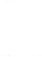
Fig. 12.3. Two instances of the knapsack problem. Left: for p = (4, 4, 1), w = (2, 2, 1), and M = 3, greedy performs better than roundDown. Right: for p = (1, M − 1) and w = (1, M), both greedy and roundDown are far from optimal
order of decreasing proÞt density and to include items that still Þt into the knapsack. We shall give this algorithm the name greedy. Figures 12.1 and 12.3 give examples. Observe that greedy always gives solutions at least as good as roundDown gives. Once roundDown encounters an item that it cannot include, it stops. However, greedy keeps on looking and often succeeds in including additional items of less weight. Although the example in Fig. 12.1 gives the same result for both greedy and roundDown, the results generally are different. For example, with proÞts p = (4, 4, 1), weights w = (2, 2, 1), and M = 3, greedy includes the Þrst and third items yielding a proÞt of 5, whereas roundDown includes just the Þrst item and obtains only a proÞt of 4. Both algorithms may produce solutions that are far from optimum. For example, for any capacity M, consider the two-item instance with proÞts p = (1, M − 1) and weights w = (1, M). Both greedy and roundDown include only the Þrst item, which has a high proÞt density but a very small absolute proÞt. In this case it would be much better to include just the second item.
We can turn this observation into an algorithm, which we call round. This computes two solutions: the solution xd proposed by roundDown and the solution xc obtained by choosing exactly the critical item x j of the fractional solution.4 It then returns the better of the two.
We can give an interesting performance guarantee. The algorithm round always achieves at least 50% of the proÞt of the optimal solution. More generally, we say that an algorithm achieves an approximation ratio of α if for all inputs, its solution is at most a factor α worse than the optimal solution.
Theorem 12.4. The algorithm round achieves an approximation ratio of 2.
Proof. Let x denote any optimal solution, and let x f be the optimal solution to the fractional knapsack problem. Then p ·x ≤ p ·x f . The value of the objective function is increased further by setting x j = 1 in the fractional solution. We obtain
p · x ≤ p · x f ≤ p · xd + p · xc ≤ 2 max p · xd , p · xc .
4We assume here that Òunreasonably largeÓ items with wi > M have been removed from the problem in a preprocessing step.
12.2 Greedy Algorithms Ð Never Look Back |
241 |
There are many ways to reÞne the algorithm round without sacriÞcing this approximation guarantee. We can replace xd by the greedy solution. We can similarly augment xc with any greedy solution for a smaller instance where item j is removed and the capacity is reduced by w j.
We now come to another important class of optimization problems, called scheduling problems. Consider the following scenario, known as the scheduling problem for independent weighted jobs on identical machines. We are given m identical machines on which we want to process n jobs; the execution of job j takes t j time units. An assignment x : 1..n → 1..m of jobs to machines is called a schedule. Thus the load j assigned to machine j is ∑{i:x(i)= j} ti. The goal is to minimize the makespan Lmax = max1≤ j≤m j of the schedule.
One application scenario is as follows. We have a video game processor with several identical processor cores. The jobs would be the tasks executed in a video game such as audio processing, preparing graphics objects for the image processing unit, simulating physical effects, and simulating the intelligence of the game.
We give next a simple greedy algorithm for the problem above [80] that has the additional property that it does not need to know the sizes of the jobs in advance. We assign jobs in the order they arrive. Algorithms with this property (Òunknown futureÓ) are called online algorithms. When job i arrives, we assign it to the machine with the smallest load. Formally, we compute the loads j = ∑h<i x(h)= j th of all machines j, and assign the new job to the least loaded machine, i.e., x(i) := ji, where ji is such that ji = min1≤ j≤m j. This algorithm is frequently referred to as the shortest-queue algorithm. It does not guarantee optimal solutions, but always computes nearly optimal solutions.
Theorem 12.5. The shortest-queue algorithm ensures that
L |
|
1 |
n |
t |
+ |
m − 1 |
max t |
. |
||
max ≤ m |
|
m |
||||||||
|
∑ i |
|
1 |
i |
n i |
|
||||
|
|
|
i=1 |
|
|
|
|
≤ ≤ |
|
|
Proof. In the schedule generated by the shortest-queue algorithm, some machine has a load Lmax. We focus on the job ıö that is the last job that has been assigned to the machine with the maximum load. When job ıö is scheduled, all m machines have a load of at least Lmax −tıö, i.e.,
∑ti ≥ (Lmax −tıö) · m .
i =ıö
Solving this for Lmax yields |
|
|
|
|
|
|
|
|
|
|
|
|
|
|
|
|
|
||||||
L |
|
1 |
∑ |
t |
+ t |
= |
|
1 |
t |
+ |
m − 1 |
t |
|
1 |
n |
t |
+ |
m − 1 |
max t |
. |
|||
max ≤ m |
m |
|
ıö ≤ m |
|
m |
||||||||||||||||||
|
i |
ıö |
|
∑ i |
|
m |
∑ i |
|
1 |
i |
n i |
|
|||||||||||
|
|
|
i |
=ıö |
|
|
|
|
i |
|
|
|
|
|
i=1 |
|
|
|
|
≤ ≤ |
|
|
|
|
|
|
|
|
|
|
|
|
|
|
|
|
|
|
|
|
|
|
|
|
|
|
|
We are almost Þnished. We now observe that ∑i ti/m and maxi ti are lower bounds on the makespan of any schedule and hence also the optimal schedule. We obtain the following corollary.

242 12 Generic Approaches to Optimization
Corollary 12.6. The approximation ratio of the shortest-queue algorithm is 2−1/m.
Proof. Let L1 = ∑i ti/m and L2 = maxi ti. The makespan of the optimal solution is at least max(L1, L2). The makespan of the shortest-queue solution is bounded by
L |
+ |
m − 1 |
L |
2 ≤ |
mL1 + (m − 1)L2 |
≤ |
(2m − 1) max(L1, L2) |
|
m |
m |
|||||
1 |
|
m |
|||||
1
= (2 − m ) · max(L1, L2) .
The shortest-queue algorithm is no better than claimed above. Consider an instance with n = m(m −1) + 1, tn = m, and ti = 1 for i < n. The optimal solution has a makespan Lmaxopt = m, whereas the shortest-queue algorithm produces a solution with a makespan Lmax = 2m − 1. The shortest-queue algorithm is an online algorithm. It produces a solution which is at most a factor 2 − 1/m worse than the solution produced by an algorithm that knows the entire input. In such a situation, we say that the online algorithm has a competitive ratio of α = 2 − 1/m.
*Exercise 12.7. Show that the shortest-queue algorithm achieves an approximation ratio of 4/3 if the jobs are sorted by decreasing size.
*Exercise 12.8 (bin packing). Suppose a smuggler boss has perishable goods in her cellar. She has to hire enough porters to ship all items tonight. Develop a greedy algorithm that tries to minimize the number of people she needs to hire, assuming that they can all carry a weight M. Try to obtain an approximation ratio for your bin-packing algorithm.
Boolean formulae provide another powerful description language. Here, variables range over the Boolean values 1 and 0, and the connectors , , and ¬ are used to build formulae. A Boolean formula is satisfiable if there is an assignment of Boolean values to the variables such that the formula evaluates to 1. As an example, we now formulate the pigeonhole principle as a satisÞability problem: it is impossible to pack n + 1 items into n bins such that every bin contains one item at most. We have variables xi j for 1 ≤ i ≤ n + 1 and 1 ≤ j ≤ n. So i ranges over items and j ranges over bins. Every item must be put into (at least) one bin, i.e., xi1 . . . xin for 1 ≤ i ≤ n + 1. No bin should receive more than one item, i.e., ¬( 1≤i<h≤n+1xi jxh j) for 1 ≤ j ≤ n. The conjunction of these formulae is unsatisÞable. SAT solvers decide the satisÞability of Boolean formulae. Although the satisÞability problem is NP-complete, there are now solvers that can solve real-world problems that involve hundreds of thousands of variables.5
Exercise 12.9. Formulate the pigeonhole principle as an integer linear program.
5 See http://www.satcompetition.org/.
12.3 Dynamic Programming Ð Building It Piece by Piece |
243 |
12.3 Dynamic Programming – Building It Piece by Piece
For many optimization problems, the following principle of optimality holds: an optimal solution is composed of optimal solutions to subproblems. If a subproblem has several optimal solutions, it does not matter which one is used.
The idea behind dynamic programming is to build an exhaustive table of optimal solutions. We start with trivial subproblems. We build optimal solutions for increasingly larger problems by constructing them from the tabulated solutions to smaller problems.
Again, we shall use the knapsack problem as an example. We deÞne P(i,C) as the maximum proÞt possible when only items 1 to i can be put in the knapsack and the total weight is at most C. Our goal is to compute P(n, M). We start with trivial cases and work our way up. The trivial cases are Òno itemsÓ and Òtotal weight zeroÓ. In both of these cases, the maximum proÞt is zero. So
P(0,C) = 0 for all C and P(i, 0) = 0 .
Consider next the case i > 0 and C > 0. In the solution that maximizes the proÞt, we either use item i or do not use it. In the latter case, the maximum achievable proÞt is P(i−1,C). In the former case, the maximum achievable proÞt is P(i−1,C −wi) + pi, since we obtain a proÞt of pi for item i and must use a solution of total weight at most C − wi for the Þrst i − 1 items. Of course, the former alternative is only feasible if C ≥ wi. We summarize this discussion in the following recurrence for P(i,C):
|
|
P(i,C) = max(P(i − 1,C), P(i − 1,C − wi) + pi) |
if wi ≤ C |
P(i − 1,C) |
if wi > C |
Exercise 12.10. Show that the case distinction in the deÞnition of P(i,C) can be avoided by deÞning P(i,C) = −∞ for C < 0.
Using the above recurrence, we can compute P(n, M) by Þlling a table P(i,C) with one column for each possible capacity C and one row for each item i. Table 12.1 gives an example. There are many ways to Þll this table, for example row by row. In order to reconstruct a solution from this table, we work our way backwards, starting at the bottom right-hand corner of the table. We set i = n and C = M. If P(i,C) = P(i −1,C), we set xi = 0 and continue to row i −1 and column C. Otherwise, we set xi = 1. We have P(i,C) = P(i − 1,C − wi) + pi, and therefore continue to row i − 1 and column C − wi. We continue with this procedure until we arrive at row 0, by which time the solution (x1, . . . , xn) has been completed.
Exercise 12.11. Dynamic programming, as described above, needs to store a table containing Θ(nM) integers. Give a more space-efÞcient solution that stores only a single bit in each table entry except for two rows of P(i,C) values at any given time. What information is stored in this bit? How is it used to reconstruct a solution? How can you get down to one row of stored values? Hint: exploit your freedom in the order of Þlling in table values.
244 12 Generic Approaches to Optimization
Table 12.1. A dynamic-programming table for the knapsack instance with p = (10, 20, 15, 20), w = (1, 3, 2, 4), and M = 5. Bold-face entries contribute to the optimal solution
i \C 0 1 |
2 |
3 |
4 |
5 |
|
0 |
0 0 |
0 |
0 |
0 |
0 |
10 10 10 10 10 10
20 10 10 20 30 30
30 10 15 25 30 35
40 10 15 25 30 35
P(i − 1,C − wi) + pi
P(i − 1,C)
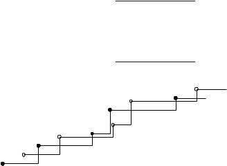
Fig. 12.4. The solid step function shows C →P(i −1,C), and the dashed step function shows C →P(i − 1,C − wi) + pi. P(i,C) is the pointwise maximum of the two functions. The solid step function is stored as the sequence of solid points. The representation of the dashed step function is obtained by adding (wi, pi) to every solid point. The representation of C →P(i,C) is obtained by merging the two representations and deleting all dominated elements
We shall next describe an important improvement with respect to space consumption and speed. Instead of computing P(i,C) for all i and all C, the Nemhauser– Ullmann algorithm [146, 17] computes only Pareto-optimal solutions. A solution x is Pareto-optimal if there is no solution that dominates it, i.e., has a greater proÞt and no greater cost or the same proÞt and less cost. In other words, since P(i,C) is an increasing function of C, only the pairs (C, P(i,C)) with P(i,C) > P(i,C − 1) are needed for an optimal solution. We store these pairs in a list Li sorted by C value. So L0 = (0, 0) , indicating that P(0,C) = 0 for all C ≥ 0, and L1 = (0, 0), (w1, p1) , indicating that P(1,C) = 0 for 0 ≤ C < w1 and P(i,C) = p1 for C ≥ w1.
How can we go from Li−1 to Li? The recurrence for P(i,C) paves the way; see Fig. 12.4. We have the list representation Li−1 for the function C →P(i − 1,C). We obtain the representation Li−1 for C →P(i − 1,C − wi) + pi by shifting every point in Li−1 by (wi, pi). We merge Li−1 and Li−1 into a single list by order of Þrst component and delete all elements that are dominated by another value, i.e., we delete all elements that are preceded by an element with a higher second component, and, for each Þxed value of C, we keep only the element with the largest second component.
Exercise 12.12. Give pseudocode for the above merge. Show that the merge can be carried out in time |Li−1|. Conclude that the running time of the algorithm is proportional to the number of Pareto-optimal solutions.