

Algorithms and data structures
.pdf142 6 Priority Queues
There are priority queues that work efficiently for integer keys. It should be noted that these queues can also be used for floating-point numbers. Indeed, the IEEE floating-point standard has the interesting property that for any valid floating-point numbers a and b, a ≤ b if and only if bits(a) ≤ bits(b), where bits(x) denotes the reinterpretation of x as an unsigned integer.
6.4.1 C++
The STL class priority_queue offers nonaddressable priority queues implemented using binary heaps. The external-memory library STXXL [48] offers an externalmemory priority queue. LEDA [118] implements a wide variety of addressable priority queues, including pairing heaps and Fibonacci heaps.
6.4.2 Java
The class java.util.PriorityQueue supports addressable priority queues to the extent that remove is implemented. However, decreaseKey and merge are not supported. Also, it seems that the current implementation of remove needs time Θ(n)! JDSL [78] offers an addressable priority queue jdsl.core.api.PriorityQueue, which is currently implemented as a binary heap.
6.5 Historical Notes and Further Findings
There is an interesting Internet survey1 of priority queues. It lists the following applications: (shortest-) path planning (see Chap. 10), discrete-event simulation, coding and compression, scheduling in operating systems, computing maximum flows, and branch-and-bound (see Sect. 12.4).
In Sect. 6.1 we saw an implementation of deleteMin by top-down search that needs about 2 log n element comparisons, and a variant using binary search that needs only log n + O(log log n) element comparisons. The latter is mostly of theoretical interest. Interestingly, a very simple “bottom-up” algorithm can be even better: The old minimum is removed and the resulting hole is sifted down all the way to the bottom of the heap. Only then, the rightmost element fills the hole and is subsequently sifted up. When used for sorting, the resulting Bottom-up heapsort requires 32 n log n + O(n) comparisons in the worst case and n log n + O(1) in the average case [204, 61, 169]. While bottom-up heapsort is simple and practical, our own experiments indicate that it is not faster than the usual top-down variant (for integer keys). This surprised us. The explanation might be that the outcomes of the comparisons saved by the bottom-up variant are easy to predict. Modern hardware executes such predictable comparisons very efficiently (see [167] for more discussion).
The recursive buildHeap routine in Exercise 6.6 is an example of a cacheoblivious algorithm [69]. This algorithm is efficient in the external-memory model even though it does not explicitly use the block size or cache size.
1 http://www.leekillough.com/heaps/survey_results.html

6.5 Historical Notes and Further Findings |
143 |
Pairing heaps [67] have constant amortized complexity for insert and merge [96] and logarithmic amortized complexity for deleteMin. The best analysis is that due to Pettie [154]. Fredman [65] has given operation sequences consisting of O(n) insertions and deleteMins and O(n log n) decreaseKeys that require time Ω(n log n log log n) for a family of addressable priority queues that includes all previously proposed variants of pairing heaps.
The family of addressable priority queues is large. Vuillemin [202] introduced binomial heaps, and Fredman and Tarjan [68] invented Fibonacci heaps. Høyer [94] described additional balancing operations that are akin to the operations used for search trees. One such operation yields thin heaps [103], which have performance guarantees similar to Fibonacci heaps and do without parent pointers and mark bits. It is likely that thin heaps are faster in practice than Fibonacci heaps. There are also priority queues with worst-case bounds asymptotically as good as the amortized bounds that we have seen for Fibonacci heaps [30]. The basic idea is to tolerate violations of the heap property and to continuously invest some work in reducing these violations. Another interesting variant is fat heaps [103].
Many applications need priority queues for integer keys only. For this special case, there are more efficient priority queues. The best theoretical bounds so far are
constant time for decreaseKey and insert and O(log log n) time for deleteMin [193,
√
136]. Using randomization, the time bound can even be reduced to O log log n [85]. The algorithms are fairly complex. However, integer priority queues that also have the monotonicity property can be simple and practical. Section 10.3 gives examples. Calendar queues [33] are popular in the discrete-event simulation community. These are a variant of the bucket queues described in Sect. 10.5.1.
7
Sorted Sequences
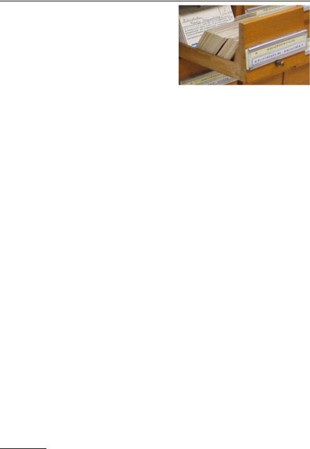
All of us spend a significant part of our time on searching, and so do computers: they look up telephone numbers, balances of bank accounts, flight reservations, bills and payments, . . . . In many applications, we want to search dynamic collections of data. New bookings are entered into reservation systems, reservations are changed or cancelled, and bookings turn into actual flights. We have already seen one solution to the problem, namely hashing. It is often desirable to keep a dynamic collection sorted. The “manual data structure” used for this purpose is a filing-card box. We can insert new cards at any position, we can remove cards, we can go through the cards in sorted order, and we can use some kind of binary search to find a particular card. Large libraries used to have filing-card boxes with hundreds of thousands of cards.1
Formally, we want to maintain a sorted sequence, i.e. a sequence of Elements sorted by their Key value, under the following operations:
•M.locate(k : Key): return min {e M : e ≥ k}.
•M.insert(e : Element): M := M {e}.
•M.remove(k : Key): M := M \ {e M : key(e) = k}.
Here, M is the set of elements stored in the sequence. For simplicity, we assume that the elements have pairwise distinct keys. We shall reconsider this assumption in Exercise 7.10. We shall show that these operations can be implemented to run in time O(log n), where n denotes the size of the sequence. How do sorted sequences compare with the data structures known to us from previous chapters? They are more flexible than sorted arrays, because they efficiently support insert and remove. They are slower but also more powerful than hash tables, since locate also works when there is no element with key k in M. Priority queues are a special case of sorted sequences; they can only locate and remove the smallest element.
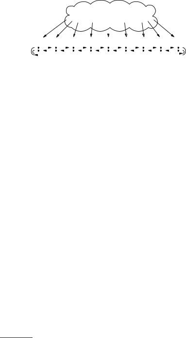
Our basic realization of a sorted sequence consists of a sorted doubly linked list with an additional navigation data structure supporting locate. Figure 7.1 illustrates this approach. Recall that a doubly linked list for n elements consists of n + 1 items,
1 The above photograph is from the catalogue of the University of Graz (Dr. M. Gossler).
146 7 Sorted Sequences
navigation data structure
|
|
|
|
|
|
|
|
|
|
|
|
|
|
|
|
|
|
|
|
|
|
|
|
|
|
2 |
|
|
3 |
|
|
5 |
|
|
7 |
|
|
11 |
|
13 |
|
17 |
|
19 |
|
∞ |
|||||
|
|
|
|
|
|
|
|
|
|
|
|
|
|
|
|
|
|
|
|
|
|
|
|
|
|
|
|
|
|
|
|
|
|
|
|
|
|
|
|
|
|
|
|
|
|
|
|
|
|
|
|
|
|
|
|
|
|
|
|
|
|
|
|
|
|
|
|
|
|
|
|
|
|
|
|
|
|
|
|
|
|
|
|
|
|
|
|
|
|
|
|
|
|
|
|
|
|
|
|
|
|
|
|
|
|
|
|
|
|
|
|
|
|
|
|
|
|
|
|
|
|
|
|
|
|
|
|
|
|
|
|
|
|
|
|
|
|
|
|
|
|
|
|
|
|
|
|
|
|
|
|
|
|
|
|
Fig. 7.1. A sorted sequence as a doubly linked list plus a navigation data structure
one for each element and one additional “dummy item”. We use the dummy item to store a special key value +∞ which is larger than all conceivable keys. We can then define the result of locate(k) as the handle to the smallest list item e ≥ k. If k is larger than all keys in M, locate will return a handle to the dummy item. In Sect. 3.1.1, we learned that doubly linked lists support a large set of operations; most of them can also be implemented efficiently for sorted sequences. For example, we “inherit” constant-time implementations for first, last, succ, and pred. We shall see constant-amortized-time implementations for remove(h : Handle), insertBefore, and insertAfter, and logarithmic-time algorithms for concatenating and splitting sorted sequences. The indexing operator [·] and finding the position of an element in the sequence also take logarithmic time. Before we delve into a description of the navigation data structure, let us look at some concrete applications of sorted sequences.
Best-first heuristics. Assume that we want to pack some items into a set of bins. The items arrive one at a time and have to be put into a bin immediately. Each item i has a weight w(i), and each bin has a maximum capacity. The goal is to minimize the number of bins used. One successful heuristic solution to this problem is to put item i into the bin that fits best, i.e., the bin whose remaining capacity is the smallest among all bins that have a residual capacity at least as large as w(i) [41]. To implement this algorithm, we can keep the bins in a sequence q sorted by their residual capacity. To place an item, we call q.locate(w(i)), remove the bin that we have found, reduce its residual capacity by w(i), and reinsert it into q. See also Exercise 12.8.
Sweep-line algorithms. Assume that you have a set of horizontal and vertical line segments in the plane and want to find all points where two segments intersect. A sweep-line algorithm moves a vertical line over the plane from left to right and maintains the set of horizontal lines that intersect the sweep line in a sorted sequence q. When the left endpoint of a horizontal segment is reached, it is inserted into q, and when its right endpoint is reached, it is removed from q. When a vertical line segment is reached at a position x that spans the vertical range [y, y ], we call s.locate(y) and scan q until we reach the key y .2 All horizontal line segments discovered during this scan define an intersection. The sweeping algorithm can be generalized to arbitrary line segments [21], curved objects, and many other geometric problems [46].
2 This range query operation is also discussed in Sect. 7.3.

7.1 Binary Search Trees |
147 |
Database indexes. A key problem in databases is to make large collections of data efficiently searchable. A variant of the (a, b)-tree data structure described in Sect. 7.2 is one of the most important data structures used for databases.
The most popular navigation data structure is that of search trees. We shall frequently use the name of the navigation data structure to refer to the entire sorted sequence data structure.3 We shall introduce search tree algorithms in three steps. As a warm-up, Sect. 7.1 introduces (unbalanced) binary search trees that support locate in O(log n) time under certain favorable circumstances. Since binary search trees are somewhat difficult to maintain under insertions and removals, we then switch to a generalization, (a, b)-trees that allows search tree nodes of larger degree. Section 7.2 explains how (a, b)-trees can be used to implement all three basic operations in logarithmic worst-case time. In Sects. 7.3 and 7.5, we shall augment search trees with additional mechanisms that support further operations. Section 7.4 takes a closer look at the (amortized) cost of update operations.
7.1 Binary Search Trees
Navigating a search tree is a bit like asking your way around in a foreign city. You ask a question, follow the advice given, ask again, follow the advice again, . . . , until you reach your destination.
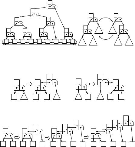
A binary search tree is a tree whose leaves store the elements of a sorted sequence in sorted order from left to right. In order to locate a key k, we start at the root of the tree and follow the unique path to the appropriate leaf. How do we identify the correct path? To this end, the interior nodes of a search tree store keys that guide the search; we call these keys splitter keys. Every nonleaf node in a binary search tree with n ≥ 2 leaves has exactly two children, a left child and a right child. The splitter key s associated with a node has the property that all keys k stored in the left subtree satisfy k ≤ s and all keys k stored in the right subtree satisfy k > s.
With these definitions in place, it is clear how to identify the correct path when locating k. Let s be the splitter key of the current node. If k ≤ s, go left. Otherwise, go right. Figure 7.2 gives an example. Recall that the height of a tree is the length of its longest root–leaf path. The height therefore tells us the maximum number of search steps needed to locate a leaf.
Exercise 7.1. Prove that a binary search tree with n ≥ 2 leaves can be arranged such that it has height log n .
A search tree with height log n is called perfectly balanced. The resulting logarithmic search time is a dramatic improvement compared with the Ω(n) time needed for scanning a list. The bad news is that it is expensive to keep perfect balance when elements are inserted and removed. To understand this better, let us consider the “naive” insertion routine depicted in Fig. 7.3. We locate the key k of the new element e before its successor e , insert e into the list, and then introduce a new node v with
3 There is also a variant of search trees where the elements are stored in all nodes of the tree.
148 |
7 |
Sorted Sequences |
|
|
|
|
|
|
|
||
|
|
|
|
|
17 |
|
|
|
|
|
|
|
|
|
7 |
|
|
|
|
|
|
|
|
|
|
3 |
|
|
13 |
|
x |
|
rotate right |
y |
|
|
|
|
|
|
|
|
|
|
|
||
2 |
|
5 |
|
11 |
19 |
|
y |
C |
A |
|
x |
|
|
|
|
|
|
||||||
2 |
3 |
5 |
7 |
11 |
13 17 19 ∞ |
A |
B |
|
rotate left |
B |
C |
Fig. 7.2. Left: the sequence 2, 3, 5, 7, 11, 13, 17, 19 represented by a binary search tree. In each node, we show the splitter key at the top and the pointers to the children at the bottom. Right: rotation of a binary search tree. The triangles indicate subtrees. Observe that the ancestor relationship between nodes x and y is interchanged
|
insert e |
|
|
u |
|
insert e |
|
u |
|
|
|
|
v |
|
|
|
v |
||
|
u |
|
|
|
u |
|
|
||
|
|
|
|
|
|
|
|
||
e |
T |
e |
e |
T |
T |
e |
T |
e |
e |
Fig. 7.3. Naive insertion into a binary search tree. A triangle indicates an entire subtree
|
insert 17 |
|
insert 13 |
|
|
insert 11 |
|
|
19 |
|||
|
|
|
|
|
|
|
19 |
|
|
|
17 |
|
|
|
|
19 |
|
|
17 |
|
|
|
13 |
|
|
19 |
|
17 |
|
|
13 |
|
|
|
11 |
|
|
|
19 |
∞ |
17 |
19 |
∞ |
13 |
17 |
19 |
∞ |
11 |
13 |
17 |
19 ∞ |
Fig. 7.4. Naively inserting sorted elements leads to a degenerate tree
left child e and right child e . The old parent u of e now points to v. In the worst case, every insertion operation will locate a leaf at the maximum depth so that the height of the tree increases every time. Figure 7.4 gives an example: the tree may degenerate to a list; we are back to scanning.
An easy solution to this problem is a healthy portion of optimism; perhaps it will not come to the worst. Indeed, if we insert n elements in random order, the expected height of the search tree is ≈ 2.99 log n [51]. We shall not prove this here, but outline a connection to quicksort to make the result plausible. For example, consider how the tree in Fig. 7.2 can be built using naive insertion. We first insert 17; this splits the set into subsets {2, 3, 5, 7, 11, 13} and {19}. From the elements in the left subset,
7.2 (a, b)-Trees and Red–Black Trees |
149 |
we first insert 7; this splits the left subset into {2, 3, 5} and {11, 13}. In quicksort terminology, we would say that 17 is chosen as the splitter in the top-level call and that 7 is chosen as the splitter in the left recursive call. So building a binary search tree and quicksort are completely analogous processes; the same comparisons are made, but at different times. Every element of the set is compared with 17. In quicksort, these comparisons take place when the set is split in the top-level call. In building a binary search tree, these comparisons take place when the elements of the set are inserted. So the comparison between 17 and 11 takes place either in the top-level call of quicksort or when 11 is inserted into the tree. We have seen (Theorem 5.6) that the expected number of comparisons in a randomized quicksort of n elements is O(n log n). By the above correspondence, the expected number of comparisons in building a binary tree by random insertions is also O(n log n). Thus any insertion requires O(log n) comparisons on average. Even more is true; with high probability each single insertion requires O(log n) comparisons, and the expected height is ≈ 2.99 log n.
Can we guarantee that the height stays logarithmic in the worst case? Yes and there are many different ways to achieve logarithmic height. We shall survey these techniques in Sect. 7.7 and discuss two solutions in detail in Sect. 7.2. We shall first discuss a solution which allows nodes of varying degree, and then show how to balance binary trees using rotations.
Exercise 7.2. Figure 7.2 indicates how the shape of a binary tree can be changed by a transformation called rotation. Apply rotations to the tree in Fig. 7.2 so that the node labelled 11 becomes the root of the tree.
Exercise 7.3. Explain how to implement an implicit binary search tree, i.e., the tree is stored in an array using the same mapping of the tree structure to array positions as in the binary heaps discussed in Sect. 6.1. What are the advantages and disadvantages compared with a pointer-based implementation? Compare searching in an implicit binary tree with binary searching in a sorted array.
7.2 (a, b)-Trees and Red–Black Trees
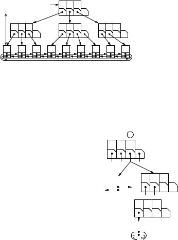
An (a, b)-tree is a search tree where all interior nodes, except for the root, have an outdegree between a and b. Here, a and b are constants. The root has degree one for a trivial tree with a single leaf. Otherwise, the root has a degree between 2 and b. For a ≥ 2 and b ≥ 2a − 1, the flexibility in node degrees allows us to efficiently maintain the invariant that all leaves have the same depth, as we shall see in a short while. Consider a node with outdegree d. With such a node, we associate an array c[1..d] of pointers to children and a sorted array s[1..d − 1] of d − 1 splitter keys. The splitters guide the search. To simplify the notation, we additionally define s[0] = −∞ and s[d] = ∞. The keys of the elements e contained in the i-th child c[i], 1 ≤ i ≤ d, lie between the i − 1-th splitter (exclusive) and the i-th splitter (inclusive), i.e., s[i −1] < key(e) ≤ s[i]. Figure 7.5 shows a (2, 4)-tree storing the sequence 2, 3, 5, 7, 11, 13, 17, 19 .
150 7 Sorted Sequences
|
|
|
|
r |
5 |
17 |
|
= 2 |
|
|
|
|
|
|
|
height |
2 |
3 |
|
|
7 |
11 13 |
19 |
|
|
|
|||||
|
2 |
3 |
5 |
7 |
11 13 |
17 19 ∞ |
|
Fig. 7.5. Representation of 2, 3, 5, 7, 11, 13, 17, 19 by a (2, 4)-tree. The tree has height 2
Class ABHandle : Pointer to ABItem or Item
// an ABItem (Item) is an item in the navigation data structure (doubly linked list)
Class ABItem(splitters : Sequence of Key, children : Sequence of ABHandle)
d = |children| : 1..b |
|
|
|
|
i |
|
|
// outdegree |
|
s = splitters : Array [1..b − 1] of Key |
1 |
2 3 |
4 |
|
|||||
c = children : Array [1..b] of Handle |
|
|
|
|
|
|
|
|
|
Function locateLocally(k : Key) : N |
7 |
11 13 |
|
k = 12 |
|||||
|
|
|
|
|
|
|
|
|
|
return min {i 1..d : k ≤ s[i]} |
|
h = 1 |
|
|
h > 1 |
||||
Function locateRec(k : Key, h : N) : Handle |
|
|
|
||||||
|
|
|
|
|
|
|
|
|
|
i:=locateLocally(k) |
|
|
|
|
|
|
12 |
||
|
|
13 |
|
|
|||||
if h = 1 then return c[i] |
|
|
|
|
|||||
|
|
|
|
|
|
|
|
|
|
else return c[i] →locateRec(k, h − 1) |
// |
|
|
|
|
|
|
|
r |
|
|
|
|
|
|
|
|||
|
|
|
|
|
|
||||
|
|
|
|
|
|
|
|||
|
|
|
|
|
|
||||
Class ABTree(a ≥ 2 : N, b ≥ 2a − 1 : N) of Element |
|
|
|
|
|
|
|
|
|
= : List of Element |
|
|
|
|
|
|
|
|
|
|
|
|
|
|
|
|
|
|
|
r : ABItem( , .head ) |
|
|
|
|
|
|
|
|
|
height = 1 : N |
|
|
// |
|
∞ |
|
|||
// Locate the smallest Item with key k ≥ k |
|
|
|
|
|
|
|
|
|
|
|
|
|
|
|
|
|
|
|
|
|
|
|
|
|
|
|
|
|
|
|
|
|
|
|
|
|
|
|
|
|
|
|
|
|
|
|
|
|
|
|
|
|
|
|
|
|
|
|
|
|
|
|
|
|
|
|
|
|
Function locate(k : Key) : Handle return r.locateRec(k, height) |
|
|
|
||||||
Fig. 7.6. (a, b)-trees. An ABItem is constructed from a sequence of keys and a sequence of handles to the children. The outdegree is the number of children. We allocate space for the maximum possible outdegree b. There are two functions local to ABItem: locateLocally(k) locates k among the splitters and locateRec(k, h) assumes that the ABItem has height h and descends h levels down the tree. The constructor for ABTree creates a tree for the empty sequence. The tree has a single leaf, the dummy element, and the root has degree one. Locating a key k in an (a, b)-tree is solved by calling r.locateRec(k, h), where r is the root and h is the height of the tree
Lemma 7.1. An (a, b)-tree for n elements has a height at most
1 + |
loga 2 |
. |
|
|
|
n + 1 |
|
7.2 (a, b)-Trees and Red–Black Trees |
151 |
Proof. The tree has n + 1 leaves, where the “+1” accounts for the dummy leaf +∞. If n = 0, the root has degree one and there is a single leaf. So, assume n ≥ 1. Let h be the height of the tree. Since the root has degree at least two and every other node has degree at least a, the number of leaves is at least 2ah−1. So n + 1 ≥ 2ah−1, or
h ≤ 1 + loga(n + 1)/2. Since the height is an integer, the bound follows. |
|
Exercise 7.4. Prove that the height of an (a, b)-tree for n elements is |
at least |
logb(n + 1) . Prove that this bound and the bound given in Lemma 7.1 are tight.
Searching in an (a, b)-tree is only slightly more complicated than searching in a binary tree. Instead of performing a single comparison at a nonleaf node, we have to find the correct child among up to b choices. Using binary search, we need at mostlog b comparisons for each node on the search path. Figure 7.6 gives pseudocode for (a, b)-trees and the locate operation. Recall that we use the search tree as a way to locate items of a doubly linked list and that the dummy list item is considered to have key value ∞. This dummy item is the rightmost leaf in the search tree. Hence, there is no need to treat the special case of root degree 0, and the handle of the dummy item can serve as a return value when one is locating a key larger than all values in the sequence.
Exercise 7.5. Prove that the total number of comparisons in a search is bounded by
log b (1 + loga(n + 1)/2). Assume b ≤ 2a. Show that this number is O(log b) + O(log n). What is the constant in front of the log n term?
To insert an element e, we first descend the tree recursively to find the smallest sequence element e ≥ e. If e and e have equal keys, e is replaced by e.
Otherwise, e is inserted into the sorted list before e . If e was the i-th child c[i] of its parent node v, then e will become the new c[i] and key(e) becomes the corresponding splitter element s[i]. The old children c[i..d] and their corresponding splitters s[i..d − 1] are shifted one position to the right. If d was less than b, d can be incremented and we are finished.
The difficult part is when a node v already has a degree d = b and now would get a degree b + 1. Let s denote the splitters of this illegal node, c its children, and
u |
u |
k |
|
||
k |
|
|
v |
t |
v |
c1 c2 c3 c4 c5 |
c1 c2 |
c3 c4 c5 |
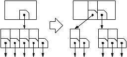
Fig. 7.7. Node splitting: the node v of degree b + 1 (here 5) is split into a node of degree(b + 1)/2 and a node of degree (b + 1)/2 . The degree of the parent increases by one. The splitter key separating the two “parts” of v is moved to the parent
152 |
7 Sorted Sequences |
|
|
|
|
|
|
|
|
|
|
|
|
|
|
|
|
r |
2 3 |
5 |
|
|
|
k = 3,t = |
|
r |
|
|
|
|
∞ |
|
|
|
2 |
|
|
5 12 |
|
2 |
3 |
5 |
|
// Example: |
|
|
|
|
|
|
|
|
|
|
// 2, 3, 5 .insert(12) |
2 |
3 |
5 |
12 |
∞ |
|
3 |
|
|
|
Procedure ABTree::insert(e : Element) |
|
|
|
|
r |
|
|
|
||
|
(k, t) := r.insertRec(e, height, ) |
|
|
|
|
|
|
|
||
|
|
|
|
|
|
|
|
|
||
|
if t =null then // root was split |
|
|
|
2 |
|
|
5 12 |
|
|
|
r := allocate ABItem( k , |
r, t ) |
|
|
|
|
|
|
|
|
|
height++ |
|
|
|
|
2 |
3 |
5 |
12 |
∞ |
|
|
|
|
|
|
|||||
// Insert a new element into a subtree of height h. |
|
|
|
|
|
|
|
|
||
//If this splits the root of the subtree,
//return the new splitter and subtree handle
Function ABItem::insertRec(e : Element, h : N, : List of Element) : Key×ABHandle |
|
||||||||||||||
i := locateLocally(e) |
|
|
|
|
|
|
|
|
|||||||
if h = 1 then |
|
// base case |
|
|
|
|
|
|
c[i] |
|
|||||
if key(c[i] → e) = key(e) then |
|
|
|
|
|
|
|
||||||||
|
|
2 |
3 |
5 |
∞ |
|
|||||||||
c[i] → e := e |
|
|
|
|
|
|
|
|
|
||||||
return ( , null ) |
|
|
|
|
|
|
e |
c[i] |
|||||||
else |
|
|
|
|
|
|
|
|
|
// 2 |
3 |
5 |
12 |
∞ |
|
(k, t) := (key(e), .insertBefore(e, c[i])) |
|||||||||||||||
else |
|
|
|
|
|
|
|
|
|
|
|
|
|
|
|
(k, t) := c[i] → insertRec(e, h − 1, ) |
|
|
|
|
|
|
|||||||||
if t = null |
then return ( , null ) |
|
s |
2 |
3 |
5 |
12 = k |
||||||||
endif |
|
|
|
|
|
|
|
|
|
c |
|
|
|
|
|
|
|
|
|
|
|
|
|
|
|
|
|
|
t |
|
|
s := s[1], . . . , s[i |
− |
1], k, s[i], . . . , s[d |
− |
1] |
|
|
|
|
∞ |
||||||
2 |
3 |
|
5 |
12 |
|||||||||||
|
|
|
|
|
|
|
|||||||||
c := c[1], . . . , c[i |
− |
1], t, c[i], . . . , c[d] |
|
// |
|
|
|
|
|
||||||
|
|
|
|
|
|
|
|
|
|
|
|
|
|||
if d < b then // there is still room here |
|
|
|
|
|
|
|||||||||
(s, c, d) := (s , c , d + 1) |
|
|
return(3, |
) |
|
|
|
||||||||
return ( , null ) |
|
|
2 |
|
|
s |
5 12 |
|
|||||||
else // split this node |
|
|
|
|
|
c |
|
|
|||||||
d := (b + 1)/2 |
|
|
2 |
3 |
|
5 |
12 |
∞ |
|||||||
s := s [b + 2 |
− |
d..b] |
|
|
|
||||||||||
|
|
|
|
|
|
|
|
|
|
|
|
|
|||
c := c [b + 2 − d..b + 1] |
|
|
// |
|
|
|
|
|
|||||||
return (s [b + 1 − d], allocate ABItem(s [1..b − d], c [1..b + 1 − d])) |
|
|
|
|
|||||||||||
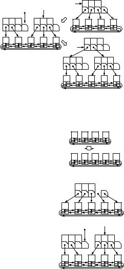
Fig. 7.8. Insertion into an (a, b)-tree
u the parent of v (if it exists). The solution is to split v in the middle (see Fig. 7.7). More precisely, we create a new node t to the left of v and reduce the degree of v to d = (b + 1)/2 by moving the b + 1 − d leftmost child pointers c [1..b + 1 − d] and the corresponding keys s [1..b − d]. The old node v keeps the d rightmost child pointers c [b + 2 − d..b + 1] and the corresponding splitters s [b + 2 − d..b].