

Algorithms and data structures
.pdf30 2 Introduction
Function factorial(n) : Z
if n = 1 then return 1 else return n · factorial(n − 1)
factorial : |
|
// |
the Þrst instruction of factorial |
Rn := RS[Rr − 1] |
|
|
// load n into register Rn |
JZ thenCase, Rn |
|
|
// jump to then case, if n is zero |
RS[Rr] = aRecCall |
// |
else case; return address for recursive call |
|
RS[Rr + 1] := Rn − 1 |
|
|
// parameter is n − 1 |
Rr := Rr + 2 |
|
|
// increase stack pointer |
J factorial |
|
|
// start recursive call |
aRecCall : |
|
// |
return address for recursive call |
Rresult := RS[Rr − 1] Rresult |
// |
store n factorial(n − 1) in result register |
|
J return |
|
|
// goto return |
thenCase : |
|
|
// code for then case |
Rresult := 1 |
|
|
// put 1 into result register |
return : |
|
|
// code for return |
Rr := Rr − 2 |
|
|
// free activation record |
J RS[Rr] |
|
|
// jump to return address |
Fig. 2.2. A recursive function factorial and the corresponding RAM code. The RAM code returns the function value in register Rresult
Rr
3
aRecCall
4
aRecCall
5
afterCall
Fig. 2.3. The recursion stack of a call factorial(5) when the recursion has reached factorial(3)
pushes the return address and the actual parameters onto the stack, increases Rr accordingly, and jumps to the Þrst instruction of the called routine called. The called routine reserves space for its local variables by increasing Rr appropriately. Then the body of called is executed. During execution of the body, any access to the i-th formal parameter (0 ≤ i < k) is an access to RS[Rr − − k + i] and any access to the i-th local variable (0 ≤ i < ) is an access to RS[Rr − + i]. When called executes a return statement, it decreases Rr by 1+ k + (observe that called knows k and ) and execution continues at the return address (which can be found at RS[Rr]). Thus control is returned to caller. Note that recursion is no problem with this scheme, since each incarnation of a routine will have its own stack area for its parameters and local variables. Figure 2.3 shows the contents of the recursion stack of a call factorial(5) when the recursion has reached factorial(3). The label afterCall is the address of the instruction following the call factorial(5), and aRecCall is deÞned in Fig. 2.2.

2.4 Designing Correct Algorithms and Programs |
31 |
Exercise 2.5 (sieve of Eratosthenes). Translate the following pseudocode for Þnding all prime numbers up to n into RAM machine code. Argue correctness Þrst.
a = 1, . . . , 1 : Array [2..n] of {0, 1} // if a[i] is false, i is known to be nonprime
√
for i := 2 to n do
if a[i] then for j := 2i to n step i do a[ j] := 0
// if a[i] is true, i is prime and all multiples of i are nonprime for i := 2 to n do if a[i] then output Òi is primeÓ
2.3.4 Object Orientation
We also need a simple form of object-oriented programming so that we can separate the interface and the implementation of the data structures. We shall introduce our notation by way of example. The deÞnition
Class Complex(x, y : Element) of Number Number r := x
Number i := y √
Function abs : Number return r2 + i2
Function add(c : Complex) : Complex return Complex(r + c .r, i + c .i)
gives a (partial) implementation of a complex number type that can use arbitrary numeric types for the real and imaginary parts. Very often, our class names will begin with capital letters. The real and imaginary parts are stored in the member variables r and i, respectively. Now, the declaration Òc : Complex(2, 3) of RÓ declares a complex number c initialized to 2 + 3i; c.i is the imaginary part, and c.abs returns the absolute value of c.
The type after the of allows us to parameterize classes with types in a way similar to the template mechanism of C++ or the generic types of Java. Note that in the light of this notation, the types ÒSet of ElementÓ and ÒSequence of ElementÓ mentioned earlier are ordinary classes. Objects of a class are initialized by setting the member variables as speciÞed in the class deÞnition.
2.4 Designing Correct Algorithms and Programs
An algorithm is a general method for solving problems of a certain kind. We describe algorithms using natural language and mathematical notation. Algorithms, as such, cannot be executed by a computer. The formulation of an algorithm in a programming language is called a program. Designing correct algorithms and translating a correct algorithm into a correct program are nontrivial and error-prone tasks. In this section, we learn about assertions and invariants, two useful concepts for the design of correct algorithms and programs.
32 2 Introduction
2.4.1 Assertions and Invariants
Assertions and invariants describe properties of the program state, i.e., properties of single variables and relations between the values of several variables. Typical properties are that a pointer has a deÞned value, an integer is nonnegative, a list is nonempty, or the value of an integer variable length is equal to the length of a certain list L. Figure 2.4 shows an example of the use of assertions and invariants in a function power(a, n0) that computes an0 for a real number a and a nonnegative integer n0.
We start with the assertion assert n0 ≥ 0 and ¬(a = 0 n0 = 0). This states that the program expects a nonnegative integer n0 and that not both a and n0 are allowed to be zero. We make no claim about the behavior of our program for inputs that violate this assertion. This assertion is therefore called the precondition of the program. It is good programming practice to check the precondition of a program, i.e., to write code which checks the precondition and signals an error if it is violated. When the precondition holds (and the program is correct), a postcondition holds at the termination of the program. In our example, we assert that r = an0 . It is also good programming practice to verify the postcondition before returning from a program. We shall come back to this point at the end of this section.
One can view preconditions and postconditions as a contract between the caller and the called routine: if the caller passes parameters satisfying the precondition, the routine produces a result satisfying the postcondition.
For conciseness, we shall use assertions sparingly, assuming that certain ÒobviousÓ conditions are implicit from the textual description of the algorithm. Much more elaborate assertions may be required for safety-critical programs or for formal veriÞcation.
Preconditions and postconditions are assertions that describe the initial and the Þnal state of a program or function. We also need to describe properties of intermediate states. Some particularly important consistency properties should hold at many places in a program. These properties are called invariants. Loop invariants and data structure invariants are of particular importance.
Function power(a : R; n0 : N) : R |
// It is not so clear what 00 should be |
assert n0 ≥ 0 and ¬(a = 0 n0 = 0) |
|
p = a : R; r = 1 : R; n = n0 : N |
// we have: pnr = an0 |
while n > 0 do |
|
invariant pnr = an0 |
|
if n is odd then n--; r := r · p |
// invariant violated between assignments |
else (n, p) := (n/2, p · p) |
// parallel assignment maintains invariant |
assert r = an0 |
// This is a consequence of the invariant and n = 0 |
return r |
|
Fig. 2.4. An algorithm that computes integer powers of real numbers
2.4 Designing Correct Algorithms and Programs |
33 |
2.4.2 Loop Invariants
A loop invariant holds before and after each loop iteration. In our example, we claim that pnr = an0 before each iteration. This is true before the Þrst iteration. The initialization of the program variables takes care of this. In fact, an invariant frequently tells us how to initialize the variables. Assume that the invariant holds before execution of the loop body, and n > 0. If n is odd, we decrement n and multiply r by p. This reestablishes the invariant (note that the invariant is violated between the assignments). If n is even, we halve n and square p, and again reestablish the invariant. When the loop terminates, we have pnr = an0 by the invariant, and n = 0 by the condition of the loop. Thus r = an0 and we have established the postcondition.
The algorithm in Fig. 2.4 and many more algorithms described in this book have a quite simple structure. A few variables are declared and initialized to establish the loop invariant. Then, a main loop manipulates the state of the program. When the loop terminates, the loop invariant together with the termination condition of the loop implies that the correct result has been computed. The loop invariant therefore plays a pivotal role in understanding why a program works correctly. Once we understand the loop invariant, it sufÞces to check that the loop invariant is true initially and after each loop iteration. This is particularly easy if the loop body consists of only a small number of statements, as in the example above.
2.4.3 Data Structure Invariants
More complex programs encapsulate their state in objects whose consistent representation is also governed by invariants. Such data structure invariants are declared together with the data type. They are true after an object is constructed, and they are preconditions and postconditions of all methods of a class. For example, we shall discuss the representation of sets by sorted arrays. The data structure invariant will state that the data structure uses an array a and an integer n, that n is the size of a, that the set S stored in the data structure is equal to {a[1], . . . , a[n]}, and that a[1] < a[2] < . . . < a[n]. The methods of the class have to maintain this invariant and they are allowed to leverage the invariant; for example, the search method may make use of the fact that the array is sorted.
2.4.4 Certifying Algorithms
We mentioned above that it is good programming practice to check assertions. It is not always clear how to do this efÞciently; in our example program, it is easy to check the precondition, but there seems to be no easy way to check the postcondition. In many situations, however, the task of checking assertions can be simplified by computing additional information. This additional information is called a certificate or witness, and its purpose is to simplify the check of an assertion. When an algorithm computes a certiÞcate for the postcondition, we call it a certifying algorithm. We shall illustrate the idea by an example. Consider a function whose input is a graph G = (V, E). Graphs are deÞned in Sect. 2.9. The task is to test whether the graph is
34 2 Introduction
bipartite, i.e., whether there is a labeling of the nodes of G with the colors blue and red such that any edge of G connects nodes of different colors. As speciÞed so far, the function returns true or false Ð true if G is bipartite, and false otherwise. With this rudimentary output, the postcondition cannot be checked. However, we may augment the program as follows. When the program declares G bipartite, it also returns a twocoloring of the graph. When the program declares G nonbipartite, it also returns a cycle of odd length in the graph. For the augmented program, the postcondition is easy to check. In the Þrst case, we simply check whether all edges connect nodes of different colors, and in the second case, we do nothing. An odd-length cycle proves that the graph is nonbipartite. Most algorithms in this book can be made certifying without increasing the asymptotic running time.
2.5 An Example – Binary Search
Binary search is a very useful technique for searching in an ordered set of items. We shall use it over and over again in later chapters.
The simplest scenario is as follows. We are given a sorted array a[1..n] of pairwise distinct elements, i.e., a[1] < a[2] < . . . < a[n], and an element x. Now we are required to Þnd the index i with a[i − 1] < x ≤ a[i]; here, a[0] and a[n + 1] should be interpreted as Þctitious elements with values −∞ and +∞, respectively. We can use these Þctitious elements in the invariants and the proofs, but cannot access them in the program.
Binary search is based on the principle of divide-and-conquer. We choose an index m [1..n] and compare x with a[m]. If x = a[m], we are done and return i = m. If x < a[m], we restrict the search to the part of the array before a[m], and if x > a[m], we restrict the search to the part of the array after a[m]. We need to say more clearly what it means to restrict the search to a subinterval. We have two indices and r, and maintain the invariant
(I) 0 ≤ < r ≤ n + 1 and a[ ] < x < a[r] .
This is true initially with = 0 and r = n + 1. If and r are consecutive indices, x is not contained in the array. Figure 2.5 shows the complete program.
The comments in the program show that the second part of the invariant is maintained. With respect to the Þrst part, we observe that the loop is entered with < r. If + 1 = r, we stop and return. Otherwise, + 2 ≤ r and hence < m < r. Thus m is a legal array index, and we can access a[m]. If x = a[m], we stop. Otherwise, we set either r = m or = m and hence have < r at the end of the loop. Thus the invariant is maintained.
Let us argue for termination next. We observe Þrst that if an iteration is not the last one, then we either increase or decrease r, and hence r − decreases. Thus the search terminates. We want to show more. We want to show that the search terminates in a logarithmic number of steps. To do this, we study the quantity r − − 1. Note that this is the number of indices i with < i < r, and hence a natural measure of the
2.5 An Example Ð Binary Search |
35 |
size of the current subproblem. We shall show that each iteration except the last at least halves the size of the problem. If an iteration is not the last, r − − 1 decreases to something less than or equal to
max{r − (r + )/2 − 1, (r + )/2 − − 1}
≤ max{r − ((r + )/2 − 1/2) − 1, (r + )/2 − − 1}
= max{(r − − 1)/2, (r − )/2 − 1} = (r − − 1)/2 ,
and hence it is at least halved. We start with r − −1 = n + 1 −0 −1 = n, and hence have r − −1 ≤ n/2k after k iterations. The (k + 1)-th iteration is certainly the last if we enter it with r = + 1. This is guaranteed if n/2k < 1 or k > log n. We conclude that, at most, 2 + log n iterations are performed. Since the number of comparisons is a natural number, we can sharpen the bound to 2 + log n .
Theorem 2.3. Binary search finds an element in a sorted array of size n in 2+ log n comparisons between elements.
Exercise 2.6. Show that the above bound is sharp, i.e., for every n there are instances where exactly 2 + log n comparisons are needed.
Exercise 2.7. Formulate binary search with two-way comparisons, i.e., distinguish between the cases x < a[m], and x ≥ a[m].
We next discuss two important extensions of binary search. First, there is no need for the values a[i] to be stored in an array. We only need the capability to compute a[i], given i. For example, if we have a strictly monotonic function f and arguments i and j with f (i) < x < f ( j), we can use binary search to Þnd m such that f (m) ≤ x < f (m + 1). In this context, binary search is often referred to as the bisection method.
Second, we can extend binary search to the case where the array is inÞnite. Assume we have an inÞnite array a[1..∞] with a[1] ≤ x and want to Þnd m such that a[m] ≤ x < a[m + 1]. If x is larger than all elements in the array, the procedure is allowed to diverge. We proceed as follows. We compare x with a[21], a[22], a[23],
. . . , until the Þrst i with x < a[2i] is found. This is called an exponential search. Then we complete the search by binary search on the array a[2i−1..2i].
( , r) := (0, n + 1) |
|
while true do |
|
invariant I |
// i.e., invariant (I) holds here |
if + 1 = r then return “a[ ] < x < a[ + 1]” |
|
m := (r + )/2 |
// < m < r |
s := compare(x, a[m]) |
// −1 if x < a[m], 0 if x = a[m], +1 if x > a[m] |
if s = 0 then return “x is equal to a[m]”; |
|
if s < 0 |
|
then r := m |
// a[ ] < x < a[m] = a[r] |
else := m |
// a[ ] = a[m] < x < a[r] |
Fig. 2.5. Binary search for x in a sorted array a[1..n]
36 2 Introduction
Theorem 2.4. The combination of exponential and binary search finds x in an unbounded sorted array in at most 2 log m + 3 comparisons, where a[m] ≤ x < a[m + 1].
Proof. We need i comparisons to Þnd the Þrst i such that x < a[2i], followed by log(2i − 2i−1) + 2 comparisons for the binary search. This gives a total of 2i + 1 comparisons. Since m ≥ 2i−1, we have i ≤ 1 + log m and the claim follows.
Binary search is certifying. It returns an index m with a[m] ≤ x < a[m + 1]. If x = a[m], the index proves that x is stored in the array. If a[m] < x < a[m + 1] and the array is sorted, the index proves that x is not stored in the array. Of course, if the array violates the precondition and is not sorted, we know nothing. There is no way to check the precondition in logarithmic time.
2.6 Basic Algorithm Analysis
Let us summarize the principles of algorithm analysis. We abstract from the complications of a real machine to the simpliÞed RAM model. In the RAM model, running time is measured by the number of instructions executed. We simplify the analysis further by grouping inputs by size and focusing on the worst case. The use of asymptotic notation allows us to ignore constant factors and lower-order terms. This coarsening of our view also allows us to look at upper bounds on the execution time rather than the exact worst case, as long as the asymptotic result remains unchanged. The total effect of these simpliÞcations is that the running time of pseudocode can be analyzed directly. There is no need to translate the program into machine code Þrst.
We shall next introduce a set of simple rules for analyzing pseudocode. Let T (I) denote the worst-case execution time of a piece of program I. The following rules then tell us how to estimate the running time for larger programs, given that we know the running times of their constituents:
•T (I; I ) = T (I) + T (I ).
•T (if C then I else I ) = O(T (C) + max(T (I), T (I ))).
•T (repeat I until C) = O ∑ki=1 T (i) , where k is the number of loop iterations, and T (i) is the time needed in the i-th iteration of the loop, including the test C.
We postpone the treatment of subroutine calls to Sect. 2.6.2. Of the rules above, only the rule for loops is nontrivial to apply; it requires evaluating sums.
2.6.1 “Doing Sums”
We now introduce some basic techniques for evaluating sums. Sums arise in the analysis of loops, in average-case analysis, and also in the analysis of randomized algorithms.
For example, the insertion sort algorithm introduced in Sect. 5.1 has two nested loops. The outer loop counts i, from 2 to n. The inner loop performs at most i − 1 iterations. Hence, the total number of iterations of the inner loop is at most

2.6 Basic Algorithm Analysis |
37 |
n |
(i |
|
1) = n−1 i = |
n(n − 1) |
= O n2 |
, |
|
∑ |
− |
||||||
2 |
|||||||
|
∑ |
|
|
||||
i=2 |
|
|
i=1 |
|
|
|
where the second equality comes from (A.11). Since the time for one execution of the inner loop is O(1), we get a worst-case execution time of Θ n2 . All nested loops with an easily predictable number of iterations can be analyzed in an analogous fashion: work your way outwards by repeatedly Þnding a closed-form expression for the innermost loop. Using simple manipulations such as ∑i cai = c ∑i ai, ∑i(ai + bi) =
∑i ai + ∑i bi, or ∑ni=2 ai = −a1 + ∑ni=1 ai, one can often reduce the sums to simple forms that can be looked up in a catalog of sums. A small sample of such formulae
can be found in Appendix A. Since we are usually interested only in the asymptotic behavior, we can frequently avoid doing sums exactly and resort to estimates. For example, instead of evaluating the sum above exactly, we may argue more simply as follows:
n |
n |
∑(i − 1) ≤ |
∑ n = n2 = O n2 , |
i=2 |
i=1 |
n |
n |
∑(i − 1) ≥ |
∑ n/2 = n/2 · n/2 = Ω n2 . |
i=2 |
i= n/2 |
|
2.6.2 Recurrences
In our rules for analyzing programs, we have so far neglected subroutine calls. Nonrecursive subroutines are easy to handle, since we can analyze the subroutine separately and then substitute the bound obtained into the expression for the running time of the calling routine. For recursive programs, however, this approach does not lead to a closed formula, but to a recurrence relation.
For example, for the recursive variant of the school method of multiplication, we obtained T (1) = 1 and T (n) = 6n + 4T ( n/2 ) for the number of prim-
itive operations. For the Karatsuba algorithm, the corresponding expression was T (n) = 3n2 + 2n for n ≤ 3 and T (n) = 12n + 3T ( n/2 + 1) otherwise. In general,
a recurrence relation deÞnes a function in terms of the same function using smaller arguments. Explicit deÞnitions for small parameter values make the function well deÞned. Solving recurrences, i.e., Þnding nonrecursive, closed-form expressions for them, is an interesting subject in mathematics. Here we focus on the recurrence relations that typically emerge from divide-and-conquer algorithms. We begin with a simple case that will sufÞce for the purpose of understanding the main ideas. We have a problem of size n = bk for some integer k. If k > 1, we invest linear work cn in dividing the problem into d subproblems of size n/b and combining the results. If k = 0, there are no recursive calls, we invest work a, and are done.
Theorem 2.5 (master theorem (simple form)). For positive constants a, b, c, and d, and n = bk for some integer k, consider the recurrence
|
if n = 1 , |
a |
|
r(n) = |
|
cn + d · r(n/b) if n > 1 .
38 2 Introduction
Then
Θ(n)
r(n) = Θ(n log n)
Θ nlogb d
if d < b ,
if d = b ,
if d > b .
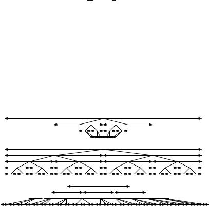
Figure 2.6 illustrates the main insight behind Theorem 2.5. We consider the amount of work done at each level of recursion. We start with a problem of size n. At the i-th level of the recursion, we have di problems, each of size n/bi. Thus the total size of the problems at the i-th level is equal to
di n = n d i . bi b
The work performed for a problem is c times the problem size, and hence the work performed at any level of the recursion is proportional to the total problem size at that level. Depending on whether d/b is less than, equal to, or larger than 1, we have different kinds of behavior.
If d < b, the work decreases geometrically with the level of recursion and the first level of recursion accounts for a constant fraction of the total execution time.
If d = b, we have the same amount of work at every level of recursion. Since there are logarithmically many levels, the total amount of work is Θ(n log n).
Finally, if d > b, we have a geometrically growing amount of work at each level of recursion so that the last level accounts for a constant fraction of the total running time. We formalize this reasoning next.
d=2, b=4
d = b = 4
d=3, b=2 


Fig. 2.6. Examples of the three cases of the master theorem. Problems are indicated by horizontal line segments with arrows at both ends. The length of a segment represents the size of the problem, and the subproblems resulting from a problem are shown in the line below it. The topmost part of Þgure corresponds to the case d = 2 and b = 4, i.e., each problem generates two subproblems of one-fourth the size. Thus the total size of the subproblems is only half of the original size. The middle part of the Þgure illustrates the case d = b = 2, and the bottommost part illustrates the case d = 3 and b = 2
2.6 Basic Algorithm Analysis |
39 |
Proof. We start with a single problem of size n = bk. W call this level zero of the recursion.3 At level 1, we have d problems, each of size n/b = bk−1. At level 2, we have d2 problems, each of size n/b2 = bk−2. At level i, we have di problems, each of size n/bi = bk−i. At level k, we have dk problems, each of size n/bk = bk−k = 1. Each such problem has a cost a, and hence the total cost at level k is adk.
Let us next compute the total cost of the divide-and-conquer steps at levels 1 to k − 1. At level i, we have di recursive calls each for subproblems of size bk−i. Each call contributes a cost of c · bk−i, and hence the cost at level i is di · c · bk−i. Thus the combined cost over all levels is
k−1 |
i |
k |
i |
k |
k−1 d i |
k−1 d i |
||||
∑ d |
· c · b |
− |
= c · b |
· ∑ |
|
|
= cn · ∑ |
|
. |
|
b |
b |
|||||||||
i=0 |
|
|
|
|
i=0 |
|
|
i=0 |
|
|
We now distinguish cases according to the relative sizes of d and b.
Case d = b. We have a cost adk = abk = an = Θ(n) for the bottom of the recursion and cnk = cn logb n = Θ(n log n) for the divide-and-conquer steps.
Case d < b. We have a cost adk < abk = an = O(n) for the bottom of the recursion.
For the cost of the divide-and-conquer steps, we use (A.13) for a geometric series, namely ∑0≤i<k xi = (1 − xk)/(1 − x) for x > 0 and x = 1, and obtain
cn |
k−1 |
d |
i = cn |
· |
1 − (d/b)k |
< cn |
· 1 |
1 |
= O(n) |
||||
|
|
− |
|
||||||||||
|
i=0 |
|
1 |
− |
d/b |
|
d/b |
|
|||||
|
· ∑ b |
|
|
|
|
|
|||||||
and |
|
|
|
|
|
|
|
|
|
|
|
|
|
cn |
k−1 |
d |
i |
= cn |
|
1 − (d/b)k |
> cn = (n) . |
|
|||||
· ∑ b |
· |
|
|
||||||||||
|
|
1 |
− |
d/b |
|
|
Ω |
|
|
||||
|
i=0 |
|
|
|
|
|
|
|
|
|
|||
Case d > b. First, note that |
|
|
|
|
|
|
|
|
|
|
|||
|
|
|
|
log b |
|
log d |
|
|
|
|
|||
dk = 2k log d = 2k log b log d = bk log b = bk logb d = nlogb d .
Hence the bottom of the recursion has a cost of anlogb d = Θ nlogb d . For the divide- and-conquer steps we use the geometric series again and obtain
cbk |
(d/b)k − 1 |
= c |
dk − bk |
= cdk |
1 − (b/d)k |
= Θ dk = Θ nlogb d . |
|
d/b − 1 |
d/b − 1 |
d/b − 1 |
|||||
|
|
|
|
We shall use the master currence T (n) = 3n2 + 2n
theorem many times in this book. Unfortunately, the refor n ≤ 3 and T (n) ≤ 12n + 3T ( n/2 + 1), governing
3In this proof, we use the terminology of recursive programs in order to give an intuitive idea of what we are doing. However, our mathematical arguments apply to any recurrence relation of the right form, even if it does not stem from a recursive program.