Algorithms and data structures

4

Hash Tables and Associative Arrays

If you want to get a book from the central library of the University of Karlsruhe, you have to order the book in advance. The library personnel fetch the book from the stacks and deliver it to a room with 100 shelves. You find your book on a shelf numbered with the last two digits of your library card. Why the last digits and not the leading digits? Probably because this distributes the books more evenly among the shelves. The library cards are numbered consecutively as students sign up, and the University of Karlsruhe was founded in 1825. Therefore, the students enrolled at the same time are likely to have the same leading digits in their card number, and only a few shelves would be in use if the leading digits were used.

The subject of this chapter is the robust and efficient implementation of the above “delivery shelf data structure”. In computer science, this data structure is known as a hash1 table. Hash tables are one implementation of associative arrays, or dictionaries. The other implementation is the tree data structures which we shall study in Chap. 7. An associative array is an array with a potentially infinite or at least very large index set, out of which only a small number of indices are actually in use. For example, the potential indices may be all strings, and the indices in use may be all identifiers used in a particular C++ program. Or the potential indices may be all ways of placing chess pieces on a chess board, and the indices in use may be the placements required in the analysis of a particular game. Associative arrays are versatile data structures. Compilers use them for their symbol table, which associates identifiers with information about them. Combinatorial search programs often use them for detecting whether a situation has already been looked at. For example, chess programs have to deal with the fact that board positions can be reached by different sequences of moves. However, each position needs to be evaluated only once. The solution is to store positions in an associative array. One of the most widely used implementations of the join operation in relational databases temporarily stores one of the participating relations in an associative array. Scripting languages such as AWK

1 Photograph of the mincer above by Kku, Rainer Zenz (Wikipedia), Licence CC-by-SA 2.5.

82 4 Hash Tables and Associative Arrays

[7] and Perl [203] use associative arrays as their main data structure. In all of the examples above, the associative array is usually implemented as a hash table. The exercises in this section ask you to develop some further uses of associative arrays.

Formally, an associative array S stores a set of elements. Each element e has an associated key key(e) Key. We assume keys to be unique, i.e., distinct elements have distinct keys. Associative arrays support the following operations:

•S.insert(e : Element): S := S {e}.

•S.remove(k : Key): S := S \ {e}, where e is the unique element with key(e) = k.

•S.find(k : Key): If there is an e S with key(e) = k, return e; otherwise, return .

In addition, we assume a mechanism that allows us to retrieve all elements in S. Since this forall operation is usually easy to implement, we discuss it only in the exercises. Observe that the find operation is essentially the random access operator for an array; hence the name “associative array”. Key is the set of potential array indices, and the elements of S are the indices in use at any particular time. Throughout this chapter, we use n to denote the size of S, and N to denote the size of Key. In a typical application of associative arrays, N is humongous and hence the use of an array of size N is out of the question. We are aiming for solutions which use space O(n).

In the library example, Key is the set of all library card numbers, and elements are the book orders. Another precomputer example is provided by an English–German dictionary. The keys are English words, and an element is an English word together with its German translations.

The basic idea behind the hash table implementation of associative arrays is simple. We use a hash function h to map the set Key of potential array indices to a small range 0..m − 1 of integers. We also have an array t with index set 0..m − 1, the hash table. In order to keep the space requirement low, we want m to be about the number of elements in S. The hash function associates with each element e a hash value h(key(e)). In order to simplify the notation, we write h(e) instead of h(key(e)) for the hash value of e. In the library example, h maps each library card number to its last two digits. Ideally, we would like to store element e in the table entry t[h(e)]. If this works, we obtain constant execution time2 for our three operations insert, remove, and find.

Unfortunately, storing e in t[h(e)] will not always work, as several elements might collide, i.e., map to the same table entry. The library example suggests a fix: allow several book orders to go to the same shelf. The entire shelf then has to be searched to find a particular order. A generalization of this fix leads to hashing with chaining. We store a set of elements in each table entry, and implement the set using singly linked lists. Section 4.1 analyzes hashing with chaining using some rather optimistic (and hence unrealistic) assumptions about the properties of the hash function. In this model, we achieve constant expected time for all three dictionary operations.

In Sect. 4.2, we drop the unrealistic assumptions and construct hash functions that come with (probabilistic) performance guarantees. Even our simple examples show

2Strictly speaking, we have to add additional terms for evaluating the hash function and for moving elements around. To simplify the notation, we assume in this chapter that all of this takes constant time.

that finding good hash functions is nontrivial. For example, if we apply the least- significant-digit idea from the library example to an English–German dictionary, we might come up with a hash function based on the last four letters of a word. But then we would have many collisions for words ending in “tion”, “able”, etc.

We can simplify hash tables (but not their analysis) by returning to the original idea of storing all elements in the table itself. When a newly inserted element e finds the entry t[h(x)] occupied, it scans the table until a free entry is found. In the library example, assume that shelves can hold exactly one book. The librarians would then use adjacent shelves to store books that map to the same delivery shelf. Section 4.3 elaborates on this idea, which is known as hashing with open addressing and linear probing.

Why are hash tables called hash tables? The dictionary defines “to hash” as “to chop up, as of potatoes”. This is exactly what hash functions usually do. For example, if keys are strings, the hash function may chop up the string into pieces of fixed size, interpret each fixed-size piece as a number, and then compute a single number from the sequence of numbers. A good hash function creates disorder and, in this way, avoids collisions.

Exercise 4.1. Assume you are given a set M of pairs of integers. M defines a binary relation RM . Use an associative array to check whether RM is symmetric. A relation is symmetric if (a, b) M : (b, a) M.

Exercise 4.2. Write a program that reads a text file and outputs the 100 most frequent words in the text.

Exercise 4.3 (a billing system). Assume you have a large file consisting of triples (transaction, price, customer ID). Explain how to compute the total payment due for each customer. Your algorithm should run in linear time.

Exercise 4.4 (scanning a hash table). Show how to realize the forall operation for hashing with chaining and for hashing with open addressing and linear probing. What is the running time of your solution?

4.1 Hashing with Chaining

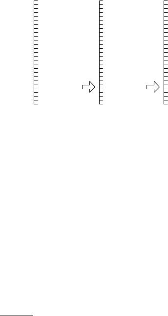
Hashing with chaining maintains an array t of linear lists (see Fig. 4.1). The associative-array operations are easy to implement. To insert an element e, we insert it somewhere in the sequence t[h(e)]. To remove an element with key k, we scan through t[h(k)]. If an element e with h(e) = k is encountered, we remove it and return. To find the element with key k, we also scan through t[h(k)]. If an element e with h(e) = k is encountered, we return it. Otherwise, we return .

Insertions take constant time. The space consumption is O(n + m). To remove or find a key k, we have to scan the sequence t[h(k)]. In the worst case, for example if find looks for an element that is not there, the entire list has to be scanned. If we are

Proof. The proof requires the probabilistic concepts of random variables, their expectation, and the linearity of expectations as described in Sect. A.3. Consider the execution time of remove or find for a fixed key k. Both need constant time plus the time for scanning the sequence t[h(k)]. Hence the expected execution time is O(1 + E[X]), where the random variable X stands for the length of the sequence t[h(k)]. Let S be the set of n elements stored in the hash table. For each e S, let Xe be the indicator variable which tells us whether e hashes to the same location as k, i.e., Xe = 1 if h(e) = h(k) and Xe = 0 otherwise. In shorthand, Xe = [h(e) = h(k)]. We have X = ∑e S Xe. Using the linearity of expectations, we obtain

E[X] = E[ ∑ Xe] = ∑ E[Xe] = ∑ prob(Xi = 1) .

e S e S e S

A random hash function maps e to all m table entries with the same probability, independent of h(k). Hence, prob(Xe = 1) = 1/m and therefore E[X] = n/m. Thus, the expected execution time of find and remove is O(1 + n/m).

We can achieve a linear space requirement and a constant expected execution time of all three operations by guaranteeing that m = Θ(n) at all times. Adaptive reallocation, as described for unbounded arrays in Sect. 3.2, is the appropriate technique.

Exercise 4.5 (unbounded hash tables). Explain how to guarantee m = Θ (n) in hashing with chaining. You may assume the existence of a hash function h : Key → N. Set h(k) = h (k) mod m and use adaptive reallocation.

Exercise 4.6 (waste of space). The waste of space in hashing with chaining is due to empty table entries. Assuming a random hash function, compute the expected number of empty table entries as a function of m and n. Hint: define indicator random variables Y0, . . . , Ym−1, where Yi = 1 if t[i] is empty.

Exercise 4.7 (average-case behavior). Assume that the hash function distributes the set of potential keys evenly over the table, i.e., for each i, 0 ≤ i ≤ m −1, we have |{k Key : h(k) = i}| ≤ N/m . Assume also that a random set S of n keys is stored in the table, i.e., S is a random subset of Key of size n. Show that for any table position i, the expected number of elements in S that hash to i is at most N/m ·n/N ≈ n/m.

4.2 Universal Hashing

Theorem 4.1 is unsatisfactory, as it presupposes that the hash function is chosen randomly from the set of all functions4 from keys to table positions. The class of all such functions is much too big to be useful. We shall show in this section that the same performance can be obtained with much smaller classes of hash functions. The families presented in this section are so small that a member can be specified in constant space. Moreover, the functions are easy to evaluate.

4We shall usually talk about a class of functions or a family of functions in this chapter, and reserve the word “set” for the set of keys stored in the hash table.

86 4 Hash Tables and Associative Arrays

Definition 4.2. Let c be a positive constant. A family H of functions from Key to 0..m − 1 is called c-universal if any two distinct keys collide with a probability of at most c/m, i.e., for all x, y in Key with x = y,

|{h H : h(x) = h(y)}| ≤ mc |H| .

In other words, for random h H,

prob(h(x) = h(y)) ≤ mc .

This definition has been constructed such that the proof of Theorem 4.1 can be extended.

Theorem 4.3. If n elements are stored in a hash table with m entries using hashing with chaining and a random hash function from a c-universal family is used, the expected execution time of remove or find is O(1 + cn/m).

Proof. We can reuse the proof of Theorem 4.1 almost word for word. Consider the execution time of remove or find for a fixed key k. Both need constant time plus the time for scanning the sequence t[h(k)]. Hence the expected execution time is O(1 + E[X]), where the random variable X stands for the length of the sequence t[h(k)]. Let S be the set of n elements stored in the hash table. For each e S, let Xe be the indicator variable which tells us whether e hashes to the same location as k, i.e., Xe = 1 if h(e) = h(k) and Xe = 0 otherwise. In shorthand, Xe = [h(e) = h(k)]. We have X = ∑e S Xe. Using the linearity of expectations, we obtain

E[X] = E[ ∑ Xe] = ∑ E[Xe] = ∑ prob(Xi = 1) .

e S e S e S

Since h is chosen uniformly from a c-universal class, we have prob(Xe = 1) ≤ c/m, and hence E[X] = cn/m. Thus, the expected execution time of find and remove is O(1 + cn/m).

Now it remains to find c-universal families of hash functions that are easy to construct and easy to evaluate. We shall describe a simple and quite practical 1- universal family in detail and give further examples in the exercises. We assume that our keys are bit strings of a certain fixed length; in the exercises, we discuss how the fixed-length assumption can be overcome. We also assume that the table size m is a prime number. Why a prime number? Because arithmetic modulo a prime is particularly nice; in particular, the set Zm = {0, . . . , m −1} of numbers modulo m form a field.5 Let w = log m . We subdivide the keys into pieces of w bits each, say k pieces. We interpret each piece as an integer in the range 0..2w − 1 and keys as k-tuples of such integers. For a key x, we write x = (x1, . . . , xk) to denote its partition

5A field is a set with special elements 0 and 1 and with addition and multiplication operations. Addition and multiplication satisfy the usual laws known for the field of rational numbers.

into pieces. Each xi lies in 0..2w −1. We can now define our class of hash functions. For each a = (a1, . . . , ak) {0..m −1}k, we define a function ha from Key to 0..m −1 as follows. Let x = (x1, . . . , xk) be a key and let a · x = ∑ki=1 aixi denote the scalar product of a and x. Then

ha(x) = a · x mod m .

It is time for an example. Let m = 17 and k = 4. Then w = 4 and we view keys as 4-tuples of integers in the range 0..15, for example x = (11, 7, 4, 3). A hash function is specified by a 4-tuple of integers in the range 0..16, for example a = (2, 4, 7, 16). Then ha(x) = (2 · 11 + 4 · 7 + 7 · 4 + 16 ·3) mod 17 = 7.

Theorem 4.4.

H· = ha : a {0..m −1}k

is a 1-universal family of hash functions if m is prime.

In other words, the scalar product between a tuple representation of a key and a random vector modulo m defines a good hash function.

Proof. Consider two distinct keys x = (x1, . . . , xk) and y = (y1, . . . , yk). To determine prob(ha(x) = ha(y)), we count the number of choices for a such that ha(x) = ha(y). Fix an index j such that x j = y j. Then (x j − y j) ≡ 0(mod m), and hence any equation of the form a j(x j − y j) ≡ b(mod m), where b Zm, has a unique solution in

inverse of (x j −y j).

We claim that for each choice of the ai’s with i = j, there is exactly one choice

i= j

a j ≡ (y j −x j)−1 ∑ ai(xi −yi) (mod m) .

i= j

There are mk−1 ways to choose the ai with i = j, and for each such choice there is a unique choice for a j. Since the total number of choices for a is mk, we obtain

Is it a serious restriction that we need prime table sizes? At first glance, yes. We certainly cannot burden users with the task of providing appropriate primes. Also, when we adaptively grow or shrink an array, it is not clear how to obtain prime

6In a field, any element z = 0 has a unique multiplicative inverse, i.e., there is a unique element z−1 such that z−1 ·z = 1. Multiplicative inverses allow one to solve linear equations of the form zx = b, where z = 0. The solution is x = z−1b.

88 4 Hash Tables and Associative Arrays

numbers for the new value of m. A closer look shows that the problem is easy to resolve. The easiest solution is to consult a table of primes. An analytical solution is not much harder to obtain. First, number theory [82] tells us that primes are abundant. More precisely, for any integer k there is a prime in the interval [k3, (k + 1)3]. So, if we are aiming for a table size of about m, we determine k such that k3 ≤ m ≤ (k + 1)3 and then search for a prime in this interval. How does this search work? Any nonprime

in the interval must have a divisor which is at most (k + 1)3 = (k + 1)3/2. We therefore iterate over the numbers from 1 to (k + 1)3/2, and for each such j remove its multiples in [k3, (k + 1)3]. For each fixed j, this takes time ((k + 1)3 − k3)/ j = O k2/ j . The total time required is

and hence is negligible compared with the cost of initializing a table of size m. The second equality in the equation above uses the harmonic sum (A.12).

Exercise 4.8 (strings as keys). Implement the universal family H· for strings. Assume that each character requires eight bits (= a byte). You may assume that the table size is at least m = 257. The time for evaluating a hash function should be proportional to the length of the string being processed. Input strings may have arbitrary lengths not known in advance. Hint: compute the random vector a lazily, extending it only when needed.

Exercise 4.9 (hashing using bit matrix multiplication). For this exercise, keys are bit strings of length k, i.e., Key = {0, 1}k, and the table size m is a power of two, say m = 2w. Each w × k matrix M with entries in {0, 1} defines a hash function hM . For x {0, 1}k, let hM (x) = Mx mod 2, i.e., hM (x) is a matrix–vector product computed modulo 2. The resulting w-bit vector is interpreted as a number in [0 . . . m −1]. Let

Hlin = hM : M {0, 1}w×k .

For M = 1 0 1 1 and x = (1, 0, 0, 1)T , we have Mx mod 2 = (0, 1)T . Note that 0 1 1 1

multiplication modulo two is the logical AND operation, and that addition modulo two is the logical exclusive-OR operation .

(a)Explain how hM (x) can be evaluated using k bit-parallel exclusive-OR operations. Hint: the ones in x select columns of M. Add the selected columns.

(b)Explain how hM (x) can be evaluated using w bit-parallel AND operations and w parity operations. Many machines provide an instruction parity(y) that returns one if the number of ones in y is odd, and zero otherwise. Hint: multiply each row of M by x.

(c)We now want to show that Hlin is 1-universal. (1) Show that for any two keys x = y, any bit position j, where x and y differ, and any choice of the columns Mi of the matrix with i = j, there is exactly one choice of a column Mj such that hM (x) = hM (y). (2) Count the number of ways to choose k − 1 columns of M.

(3) Count the total number of ways to choose M. (4) Compute the probability prob(hM (x) = hM (y)) for x = y if M is chosen randomly.

*Exercise 4.10 (more matrix multiplication). Define a class of hash functions

H× = hM : M {0.. p −1}w×k

that generalizes the class Hlin by using arithmetic modulo p for some prime number p. Show that H× is 1-universal. Explain how H· is a special case of H×.

Exercise 4.11 (simple linear hash functions). Assume that Key = 0.. p − 1 = Zp

for some prime number p. For a, b Zp, let h(a,b)(x) = ((ax + b) mod p) mod m, and m ≤ p. For example, if p = 97 and m = 8, we have h(23,73)(2) = ((23 · 2 + 73) mod 97) mod 8 = 22 mod 8 = 6. Let

H = h(a,b) : a, b 0.. p −1 .

Show that this family is ( p/m /( p/m))2-universal.

Exercise 4.12 (continuation). Show that the following holds for the class H defined

in the previous exercise. For any pair of distinct keys x and y and any i and j in 0..m −1, prob(h(a,b)(x) = i and h(a,b)(y) = j) ≤ c/m2 for some constant c.

Exercise 4.13 (a counterexample). Let Key = 0.. p −1, and consider the set of hash

functions

Hfool = h(a,b) : a, b 0.. p −1

with h(a,b)(x) = (ax + b) mod m. Show that there is a set S of p/m keys such that for any two keys x and y in S, all functions in Hfool map x and y to the same value. Hint: let S = {0, m, 2m, . . . , p/m m}.

Exercise 4.14 (table size 2 ). Let Key = 0..2k − 1. Show that the family of hash functions

H = ha : 0 < a < 2k a is odd

with ha(x) = (ax mod 2k) div 2k− is 2-universal. Hint: see [53].

Exercise 4.15 (table lookup). Let m = 2w, and view keys as k + 1-tuples, where the zeroth element is a w-bit number and the remaining elements are a-bit numbers for some small constant a. A hash function is defined by tables t1 to tk, each having a size s = 2a and storing bit strings of length w. We then have

90 4 Hash Tables and Associative Arrays

k

h (t1,...,tk)((x0, x1, . . . , xk)) = x0 ti[xi] ,

i=1

i.e., xi selects an element in table ti, and then the bitwise exclusive-OR of x0 and the ti[xi] is formed. Show that

H [] = h(t1,...,tk) : ti {0..m −1}s

is 1-universal.

4.3 Hashing with Linear Probing

Hashing with chaining is categorized as a closed hashing approach because each table entry has to cope with all elements hashing to it. In contrast, open hashing schemes open up other table entries to take the overflow from overloaded fellow entries. This added flexibility allows us to do away with secondary data structures such as linked lists – all elements are stored directly in table entries. Many ways of organizing open hashing have been investigated [153]. We shall explore only the simplest scheme. Unused entries are filled with a special element . An element e is stored in the entry t[h(e)] or further to the right. But we only go away from the index h(e) with good reason: if e is stored in t[i] with i > h(e), then the positions h(e) to i −1 are occupied by other elements.

The implementations of insert and find are trivial. To insert an element e, we linearly scan the table starting at t[h(e)], until a free entry is found, where e is then stored. Figure 4.2 gives an example. Similarly, to find an element e, we scan the table, starting at t[h(e)], until the element is found. The search is aborted when an empty table entry is encountered. So far, this sounds easy enough, but we have to deal with one complication. What happens if we reach the end of the table during an insertion? We choose a very simple fix by allocating m table entries to the right of the largest index produced by the hash function h. For “benign” hash functions, it should be sufficient to choose m much smaller than m in order to avoid table overflows. Alternatively, one may treat the table as a cyclic array; see Exercise 4.16 and Sect. 3.4. This alternative is more robust but slightly slower.

The implementation of remove is nontrivial. Simply overwriting the element with does not suffice, as it may destroy the invariant. Assume that h(x) = h(z), h(y) = h(x) + 1, and x, y, and z are inserted in this order. Then z is stored at position h(x) + 2. Overwriting y with will make z inaccessible. There are three solutions. First, we can disallow removals. Second, we can mark y but not actually remove it. Searches are allowed to stop at , but not at marked elements. The problem with this approach is that the number of nonempty cells (occupied or marked) keeps increasing, so that searches eventually become slow. This can be mitigated only by introducing the additional complication of periodic reorganizations of the table. Third, we can actively restore the invariant. Assume that we want to remove the element at i. We overwrite it with leaving a “hole”. We then scan the entries to the right