

Algorithms and data structures
.pdf5.4 Quicksort |
111 |
5.4.2 *Refinements
We shall now discuss reÞnements of the basic quicksort algorithm. The resulting algorithm, called qsort, works in-place, and is fast and space-efÞcient. Figure 5.7 shows the pseudocode, and Figure 5.8 shows a sample execution. The reÞnements are nontrivial and we need to discuss them carefully.
Procedure qSort(a : Array of Element; , r : N) |
// Sort the subarray a[ ..r] |
||||||
while r − + 1 > n0 do |
|
// Use divide-and-conquer. |
|||||
j := pickPivotPos(a, , r) |
// Pick a pivot element and |
||||||
swap(a[ ], a[ j]) |
|
// bring it to the Þrst position. |
|||||
p := a[ ] |
|
|
|
|
// p is the pivot now. |
||
i := ; j := r |
|
|
|
|
|
|
|
repeat |
|
// a: |
|
|
i→ ←j |
r |
|
|
|
|
|||||
while a[i ] < p do i++ |
|
|
// Skip over elements |
||||
while a[ j] > p do j-- |
// already in the correct subarray. |
||||||
if i ≤ j then |
|
// If partitioning is not yet complete, |
|||||
swap(a[i], a[ j]); i++; j-- |
// (*) swap misplaced elements and go on. |
||||||
until i > j |
|
// Partitioning is complete. |
|||||
if i < ( + r)/2 then |
qSort(a, , j); := i |
|
|
|
// Recurse on |
||
else |
qSort(a, i, r); r := j |
// |
smaller subproblem. |
||||
endwhile |
|
|
|
|
faster for small r − |
||
insertionSort(a[ ..r]) |
|
// |
|||||
Fig. 5.7. ReÞned quicksort for arrays
The function qsort operates on an array a. The arguments and r specify the subarray to be sorted. The outermost call is qsort(a, 1, n). If the size of the subproblem is smaller than some constant n0, we resort to a simple algorithm3 such as the insertion sort shown in Fig. 5.1. The best choice for n0 depends on many details of the machine and compiler and needs to be determined experimentally; a value somewhere between 10 and 40 should work Þne under a variety of conditions.
The pivot element is chosen by a function pickPivotPos that we shall not specify further. The correctness does not depend on the choice of the pivot, but the efÞciency does. Possible choices are the Þrst element; a random element; the median (ÒmiddleÓ) element of the Þrst, middle, and last elements; and the median of a random sample
consisting of k elements, where k is either a small constant, say three, or a number |
|
depending on the problem size, say √r − + 1 |
. The Þrst choice requires the least |
amount of work, but gives little control over the size of the subproblems; the last choice requires a nontrivial but still sublinear amount of work, but yields balanced
3Some authors propose leaving small pieces unsorted and cleaning up at the end using a single insertion sort that will be fast, according to Exercise 5.7. Although this nice trick reduces the number of instructions executed, the solution shown is faster on modern machines because the subarray to be sorted will already be in cache.
112 |
5 Sorting and Selection |
|
|
|
|
|
|
|
|
|
|||
i → |
|
← j |
3 6 8 1 0 7 2 4 5 9 |
||||||||||
3 |
6 |
8 1 0 7 2 4 |
5 |
9 |
2 |
0 |
1|8 |
6 |
7 |
3 |
4 |
5 |
9 |
2 |
6 |
8 1 0 7 3 4 |
5 |
9 |
1 |
|
| |
6 |
7 |
3 |
4|8 |
9 |
|
0|2|5 |
|||||||||||||
2 |
0 |
8 1 6 7 3 4 |
5 |
9 |
0 |
| |
| |
3|7 |
6 |
| |
|
9 |
|
1| |
|4 |
5|8 |
|||||||||||
2 |
0 |
1 8 6 7 3 4 |
5 |
9 |
|
| |
| |
|
| |
|
| |
|
|
|
| |
|3 |
4|5 |
6|7| |
|
|
|||||||
|
|
j i |
|
|
|
| |
| |
|
| |
|
| | |
|
|
|
|
|
|
|
| |
| |
|
|5 |
6| | |
|
|
||
Fig. 5.8. Execution of qSort (Fig. 5.7) on 3, 6, 8, 1, 0, 7, 2, 4, 5, 9 using the Þrst element as the pivot and n0 = 1. The left-hand side illustrates the Þrst partitioning step, showing elements in bold that have just been swapped. The right-hand side shows the result of the recursive partitioning operations
subproblems with high probability. After selecting the pivot p, we swap it into the Þrst position of the subarray (= position of the full array).
The repeatÐuntil loop partitions the subarray into two proper (smaller) subarrays. It maintains two indices i and j. Initially, i is at the left end of the subarray and j is at the right end; i scans to the right, and j scans to the left. After termination of the loop, we have i = j + 1 or i = j + 2, all elements in the subarray a[.. j] are no larger than p, all elements in the subarray a[i..r] are no smaller than p, each subarray is a proper subarray, and, if i = j + 2, a[i + 1] is equal to p. So, recursive calls qSort(a, , j) and qsort(a, i, r) will complete the sort. We make these recursive calls in a nonstandard fashion; this is discussed below.
Let us see in more detail how the partitioning loops work. In the Þrst iteration of the repeat loop, i does not advance at all but remains at , and j moves left to the rightmost element no larger than p. So j ends at or at a larger value; generally, the latter is the case. In either case, we have i ≤ j. We swap a[i] and a[ j], increment i, and decrement j. In order to describe the total effect more generally, we distinguish cases.
If p is the unique smallest element of the subarray, j moves all the way to , the swap has no effect, and j = − 1 and i = + 1 after the increment and decrement. We have an empty subproblem .. − 1 and a subproblem + 1..r. Partitioning is complete, and both subproblems are proper subproblems.
If j moves down to i + 1, we swap, increment i to + 1, and decrement j to. Partitioning is complete, and we have the subproblems .. and + 1..r. Both subarrays are proper subarrays.
If j stops at an index larger than i + 1, we have < i ≤ j < r after executing the line in Fig. 5.7 marked (*). Also, all elements left of i are at most p (and there is at least one such element), and all elements right of j are at least p (and there is at least one such element). Since the scan loop for i skips only over elements smaller than p and the scan loop for j skips only over elements larger than p, further iterations of the repeat loop maintain this invariant. Also, all further scan loops are guaranteed to terminate by the claims in parentheses and so there is no need for an index-out- of-bounds check in the scan loops. In other words, the scan loops are as concise as possible; they consist of a test and an increment or decrement.
5.4 Quicksort |
113 |
Let us next study how the repeat loop terminates. If we have i ≤ j + 2 after the scan loops, we have i ≤ j in the termination test. Hence, we continue the loop. If we have i = j − 1 after the scan loops, we swap, increment i, and decrement j. So i = j + 1, and the repeat loop terminates with the proper subproblems .. j and i..r. The case i = j after the scan loops can occur only if a[i] = p. In this case, the swap has no effect. After incrementing i and decrementing j, we have i = j + 2, resulting in the proper subproblems .. j and j + 2..r, separated by one occurrence of p. Finally, when i > j after the scan loops, then either i goes beyond j in the Þrst scan loop, or j goes below i in the second scan loop. By our invariant, i must stop at j + 1 in the Þrst case, and then j does not move in its scan loop or j must stop at i − 1 in the second case. In either case, we have i = j + 1 after the scan loops. The line marked
(*) is not executed, so that we have subproblems .. j and i..r, and both subproblems are proper.
We have now shown that the partitioning step is correct, terminates, and generates proper subproblems.
Exercise 5.22. Is it safe to make the scan loops skip over elements equal to p? Is this safe if it is known that the elements of the array are pairwise distinct?
The reÞned quicksort handles recursion in a seemingly strange way. Recall that we need to make the recursive calls qSort(a, , j) and qSort(a, i, r). We may make these calls in either order. We exploit this ßexibility by making the call for the smaller subproblem Þrst. The call for the larger subproblem would then be the last thing done in qSort. This situation is known as tail recursion in the programming-language literature. Tail recursion can be eliminated by setting the parameters ( and r) to the right values and jumping to the Þrst line of the procedure. This is precisely what the while loop does. Why is this manipulation useful? Because it guarantees that the recursion stack stays logarithmically bounded; the precise bound is log(n/n0) . This follows from the fact that we make a single recursive call for a subproblem which is at most half the size.
Exercise 5.23. What is the maximal depth of the recursion stack without the Òsmaller subproblem ÞrstÓ strategy? Give a worst-case example.
*Exercise 5.24 (sorting strings using multikey quicksort [22]). Let s be a sequence of n strings. We assume that each string ends in a special character that is different from all ÒnormalÓ characters. Show that the function mkqSort(s, 1) below sorts a sequence s consisting of different strings. What goes wrong if s contains equal strings? Solve this problem. Show that the expected execution time of mkqSort is O(N + n log n) if N = ∑e s |e|.
Function mkqSort(s : Sequence of String, i : N) : Sequence of String
assert e, e s : e[1..i − 1] = e [1..i − 1] |
|
if |s| ≤ 1 then return s |
// base case |
pick p s uniformly at random |
// pivot character |
return concatenation of mkqSort( e s : e[i] < p[i] , i), mkqSort( e s : e[i] = p[i] , i + 1), and mkqSort( e s : e[i] > p[i] , i)
114 5 Sorting and Selection
Exercise 5.25. Implement several different versions of qSort in your favorite programming language. Use and do not use the reÞnements discussed in this section, and study the effect on running time and space consumption.
5.5 Selection
Selection refers to a class of problems that are easily reduced to sorting but do not require the full power of sorting. Let s = e1, . . . , en be a sequence and call its sorted version s = e1, . . . , en . Selection of the smallest element requires determining e1, selection of the largest requires determining en, and selection of the k-th smallest requires determining ek. Selection of the median refers to selecting e n/2 . Selection of the median and also of quartiles is a basic problem in statistics. It is easy to determine the smallest element or the smallest and the largest element by a single scan of a sequence in linear time. We now show that the k-th smallest element can also be determined in linear time. The simple recursive procedure shown in Fig. 5.9 solves the problem.
This procedure is akin to quicksort and is therefore called quickselect. The key insight is that it sufÞces to follow one of the recursive calls. As before, a pivot is chosen, and the input sequence s is partitioned into subsequences a, b, and c containing the elements smaller than the pivot, equal to the pivot, and larger than the pivot, respectively. If |a| ≥ k, we recurse on a, and if k > |a| + |b|, we recurse on c with a suitably adjusted k. If |a| < k ≤ |a| + |b|, the task is solved: the pivot has rank k and we return it. Observe that the latter case also covers the situation |s| = k = 1, and hence no special base case is needed. Figure 5.10 illustrates the execution of quickselect.
// Find an element with rank k |
|
|
|
|
|
|
|
|
|
|
|
|
Function select(s : Sequence of Element; k : N) : Element |
|
|
|
|
|
|
||||||
assert |s| ≥ k |
|
|
|
|
|
|
|
|
// pivot key |
|||
pick p s uniformly at random |
|
|
|
|
|
|
|
|
||||
a := e s : e < p |
|
|
|
|
|
|
|
|
|
|
k |
|
if |a| ≥ k then return select(a, k) |
|
|
// |
|
a |
|
||||||
b := e s : e = p |
|
|
|
|
|
|
|
|
|
|
k |
|
if |a| + |b| ≥ k then return p |
|
|
|
|
|
// |
a |
b = p, . . . , p |
||||
c := e s : e > p |
|
|
|
|
|
|
|
|
|
|
k |
|
return select(c, k − |a| − |b|) |
|
|
|
|
|
// |
a |
|
b |
c |
||
|
|
|
|
|
|
|
|
|||||
|
|
Fig. 5.9. Quickselect |
|
|
|
|
|
|
||||
|
s |
k |
|
p |
a |
b |
|
c |
|
|
|
|
|
|
|
|
|
|
|||||||
|
|
|
|
|
|
|
|
|||||
3, 1, 4, 5, 9, 2, 6, 5, 3, 5, 8 6 |
|
2 |
1 |
2 3, 4, 5, 9, 6, 5, 3, 5, 8 |
|
|
||||||
3, 4, 5, 9, 6, 5, 3, 5, 8 |
4 |
|
6 3, 4, 5, 5, 3, 4 6 |
|
9, 8 |
|
|
|
|
|||
3, 4, 5, 5, 3, 5 |
4 |
|
5 |
3, 4, 3 |
5, 5, 5 |
|
|
|
|
|
|
|
Fig. 5.10. The execution of select( 3, 1, 4, 5, 9, 2, 6, 5, 3, 5, 8, 6 , 6). The middle element (bold) of the current s is used as the pivot p

5.5 Selection |
115 |
As for quicksort, the worst-case execution time of quickselect is quadratic. But the expected execution time is linear and hence is a logarithmic factor faster than quicksort.
Theorem 5.8. The quickselect algorithm runs in expected time O(n) on an input of size n.
Proof. We shall give an analysis that is simple and shows a linear expected execution time. It does not give the smallest constant possible. Let T (n) denote the expected execution time of quickselect. We call a pivot good if neither |a| nor |c| is larger than 2n/3. Let γ denote the probability that a pivot is good; then γ ≥ 1/3. We now make the conservative assumption that the problem size in the recursive call is reduced only for good pivots and that, even then, it is reduced only by a factor of 2/3. Since the work outside the recursive call is linear in n, there is an appropriate constant c such that
|
|
|
|
|
|
|
|
|
|
|
2n |
|
|
|
|
|
|
|
||
|
|
T (n) ≤ cn + γ T |
|
|
|
+ (1 − γ )T (n) . |
|
|
|
|
||||||||||
|
|
|
3 |
|
|
|
|
|
||||||||||||
Solving for T (n) yields |
|
|
|
|
|
|
|
|
|
|
|
|
|
|
|
|
|
|||
|
cn |
|
2n |
|
|
|
|
|
2n |
|
2n |
|
4n |
|
||||||
T (n) ≤ |
|
+ T |
|
|
|
|
≤ 3cn + T |
|
≤ 3c n + |
|
+ |
|
|
+ . . . |
||||||
γ |
|
3 |
|
3 |
3 |
9 |
||||||||||||||
≤ 3cn ∑ |
|
2 |
i |
|
|
1 |
|
|
= 9cn . |
|
|
|
|
|
||||||
|
|
|
≤ 3cn |
|
|
|
|
|
|
|
|
|||||||||
|
3 |
|
1 |
− |
2/3 |
|
|
|
|
|
||||||||||
|
|
i≥0 |
|
|
|
|
|
|
|
|
|
|
|
|
|
|
|
|
||
Exercise 5.26. Modify quickselect so that it returns the k smallest elements.
Exercise 5.27. Give a selection algorithm that permutes an array in such a way that the k smallest elements are in entries a[1], . . . , a[k]. No further ordering is required except that a[k] should have rank k. Adapt the implementation tricks used in the array-based quicksort to obtain a nonrecursive algorithm with fast inner loops.
Exercise 5.28 (streaming selection).
(a)Develop an algorithm that Þnds the k-th smallest element of a sequence that is presented to you one element at a time in an order you cannot control. You have only space O(k) available. This models a situation where voluminous data arrives over a network or at a sensor.
(b)ReÞne your algorithm so that it achieves a running time O(n log k). You may want to read some of Chap. 6 Þrst.
*(c) ReÞne the algorithm and its analysis further so that your algorithm runs in average-case time O(n) if k = O(n/ log n). Here, ÒaverageÓ means that all orders of the elements in the input sequence are equally likely.

116 5 Sorting and Selection
5.6 Breaking the Lower Bound
The title of this section is, of course, nonsense. A lower bound is an absolute statement. It states that, in a certain model of computation, a certain task cannot be carried out faster than the bound. So a lower bound cannot be broken. But be careful. It cannot be broken within the model of computation used. The lower bound does not exclude the possibility that a faster solution exists in a richer model of computation. In fact, we may even interpret the lower bound as a guideline for getting faster. It tells us that we must enlarge our repertoire of basic operations in order to get faster.
What does this mean in the case of sorting? So far, we have restricted ourselves to comparison-based sorting. The only way to learn about the order of items was by comparing two of them. For structured keys, there are more effective ways to gain information, and this will allow us to break the Ω(n log n) lower bound valid for comparison-based sorting. For example, numbers and strings have structure; they are sequences of digits and characters, respectively.
Let us start with a very simple algorithm Ksort that is fast if the keys are small integers, say in the range 0..K − 1. The algorithm runs in time O(n + K). We use an array b[0..K − 1] of buckets that are initially empty. We then scan the input and insert an element with key k into bucket b[k]. This can be done in constant time per element, for example by using linked lists for the buckets. Finally, we concatenate all the nonempty buckets to obtain a sorted output. Figure 5.11 gives the pseudocode. For example, if the elements are pairs whose Þrst element is a key in the range 0..3 and
s = (3, a), (1, b), (2, c), (3, d), (0, e), (0, f ), (3, g), (2, h), (1, i) ,
we obtain b = [ (0, e), (0, f ) , (1, b), (1, i) , (2, c), (2, h) , (3, a), (3, d), (3, g) ] and output (0, e), (0, f ), (1, b), (1, i), (2, c), (2, h), (3, a), (3, d), (3, g) . This example illustrates an important property of Ksort. It is stable, i.e., elements with the same key inherit their relative order from the input sequence. Here, it is crucial that elements are appended to their respective bucket.
KSort can be used as a building block for sorting larger keys. The idea behind radix sort is to view integer keys as numbers represented by digits in the range 0..K −1. Then KSort is applied once for each digit. Figure 5.12 gives a radix-sorting algorithm for keys in the range 0..Kd − 1 that runs in time O(d(n + K)). The elements are Þrst sorted by their least signiÞcant digit (LSD radix sort), then by the second least signiÞcant digit, and so on until the most signiÞcant digit is used for sorting. It is not obvious why this works. The correctness rests on the stability of
Procedure KSort(s : Sequence of Element)
b = , . . . , : Array [0..K − 1] of Sequence of Element foreach e s do b[key(e)].pushBack(e)
s := concatenation of b[0], . . . , b[K − 1]
s  e
e
//
b[0] b[1] b[2] b[3] b[4]
Fig. 5.11. Sorting with keys in the range 0..K − 1

5.6 Breaking the Lower Bound |
117 |
Procedure LSDRadixSort(s : Sequence of Element) for i := 0 to d − 1 do
redeÞne key(x) as (x div Ki) mod K KSort(s)
invariant s is sorted with respect to digits i..0
|
|
... |
digits |
... |
|
|
|
// x |
d−1 |
i |
|
1 |
0 |
||
|
|
|
key(x |
) |
|
|
|
Fig. 5.12. Sorting with keys in 0..Kd − 1 using least signiÞcant digit (LSD) radix sort
Procedure uniformSort(s : Sequence of Element) n := |s|
b = , . . . , : Array [0..n − 1] of Sequence of Element foreach e s do b[ key(e) · n ].pushBack(e)
for i := 0 to n − 1 do sort b[i] in time O(|b[i]|log |b[i]|) s := concatenation of b[0], . . . , b[n − 1]
Fig. 5.13. Sorting random keys in the range [0, 1)
Ksort. Since KSort is stable, the elements with the same i-th digit remain sorted with respect to digits i − 1..0 during the sorting process with respect to digit i. For example, if K = 10, d = 3, and
s = 017, 042, 666, 007, 111, 911, 999 , we successively obtain s = 111, 911, 042, 666, 017, 007, 999 ,
s = 007, 111, 911, 017, 042, 666, 999 , and
s = 007, 017, 042, 111, 666, 911, 999 .
Radix sort starting with the most signiÞcant digit (MSD radix sort) is also possible. We apply KSort to the most signiÞcant digit and then sort each bucket recursively. The only problem is that the buckets might be much smaller than K, so that it would be expensive to apply KSort to small buckets. We then have to switch to another algorithm. This works particularly well if we can assume that the keys are uniformly distributed. More speciÞcally, let us now assume that the keys are real numbers with 0 ≤ key(e) < 1. The algorithm uniformSort in Fig. 5.13 scales these keys to integers between 0 and n − 1 = |s| − 1, and groups them into n buckets, where bucket b[i] is responsible for keys in the range [i/n, (i + 1)/n). For example, if s = 0.8, 0.4, 0.7, 0.6, 0.3 , we obtain Þve buckets responsible for intervals of size 0.2, and
b = [ , 0.3 , 0.4 , 0.7, 0.6 , 0.8 ] ;
only b[3] = 0.7, 0.6 is a nontrivial subproblem. uniformSort is very efÞcient for random keys.
Theorem 5.9. If the keys are independent uniformly distributed random values in [0, 1), uniformSort sorts n keys in expected time O(n) and worst-case time O(n log n).

118 5 Sorting and Selection
Proof. We leave the worst-case bound as an exercise and concentrate on the average case. The total execution time T is O(n) for setting up the buckets and concatenating the sorted buckets, plus the time for sorting the buckets. Let Ti denote the time for sorting the i-th bucket. We obtain
E [T ] = O(n) + E ∑ Ti |
= O(n) + ∑ E[Ti] = O(n) + nE[T0] . |
i<n |
i<n |
The second equality follows from the linearity of expectations (A.2), and the third equality uses the fact that all bucket sizes have the same distribution for uniformly distributed inputs. Hence, it remains to show that E[T0] = O(1). We shall prove the stronger claim that E[T0] = O(1) even if a quadratic-time algorithm such as insertion sort is used for sorting the buckets. The analysis is similar to the arguments used to analyze the behavior of hashing in Chap. 4.
Let B0 = |b[0]|. We have E[T0] = O E[B20] . The random variable B0 obeys a binomial distribution (A.7) with n trials and success probability 1/n, and hence
n 1 i |
1 n−i |
|
ni 1 |
1 |
|
|
e |
i |
||||||
prob(B0 = i) = i |
|
|
1 − |
|
|
≤ |
|
|
= |
|
≤ |
|
|
|
n |
|
n |
|
i! |
ni |
i! |
|
i |
, |
|||||
where the last inequality follows from StirlingÕs approximation to the factorial (A.9). We obtain
2 |
] = ∑ i |
2 |
|
|
|
= i) ≤ ∑ i |
2 |
e i |
||||||||
E[B0 |
|
prob(B0 |
|
|
|
|
||||||||||
|
|
|
i |
|||||||||||||
|
i≤n |
|
|
|
|
|
|
|
|
|
i≤n |
|
|
|
|
|
|
≤ ∑ i |
2 e i |
|
2 |
∑ |
e i−2 |
||||||||||
|
|
|
|
+ e |
|
|
|
|
|
|
|
|
||||
|
|
|
i |
|
|
i |
|
|
|
|
||||||
|
i≤5 |
|
|
|
|
|
|
i≥6 |
|
|
|
|
|
|
|
|
|
≤ O(1) + e2 ∑ |
1 |
i−2 = O(1) , |
|||||||||||||
|
2 |
|||||||||||||||
|
|
|
|
|
i≥6 |
|
|
|
|
|
|
|
|
|
|
|
and hence E[T ] = O(n) (note that the split at i = 6 allows us to conclude that e/i ≤ 1/2).
*Exercise 5.29. Implement an efÞcient sorting algorithm for elements with keys in the range 0..K − 1 that uses the data structure of Exercise 3.20 for the input and output. The space consumption should be n + O(n/B + KB) for n elements, and blocks of size B.
5.7 *External Sorting
Sometimes the input is so huge that it does not Þt into internal memory. In this section, we shall learn how to sort such data sets in the external-memory model introduced in Sect. 2.2. This model distinguishes between a fast internal memory of size M and a large external memory. Data is moved in the memory hierarchy in
|
|
|
5.7 |
*External Sorting |
119 |
make_things_ |
as_simple_as _possible_bu t_no_simpler |
|
|||
formRuns |
|
formRuns |
formRuns |
formRuns |
|
__aeghikmnst |
__aaeilmpsss __aaeilmpsss __eilmnoprst |
|
|||
|
merge |
merge |
|
||
____aaaeeghiiklmmnpsssst ____bbeeiillmnoopprssstu
merge
________aaabbeeeeghiiiiklllmmmnnooppprsssssssttu
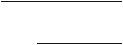
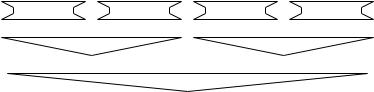
Fig. 5.14. An example of two-way mergesort with initial runs of length 12
blocks of size B. Scanning data is fast in external memory and mergesort is based on scanning. We therefore take mergesort as the starting point for external-memory sorting.
Assume that the input is given as an array in external memory. We shall describe a nonrecursive implementation for the case where the number of elements n is divisible by B. We load subarrays of size M into internal memory, sort them using our favorite algorithm, for example qSort, and write the sorted subarrays back to external memory. We refer to the sorted subarrays as runs. The run formation phase takes n/B block reads and n/B block writes, i.e., a total of 2n/B I/Os. We then merge pairs of runs into larger runs in log(n/M) merge phases, ending up with a single sorted run. Figure 5.14 gives an example for n = 48 and runs of length 12.
How do we merge two runs? We keep one block from each of the two input runs and from the output run in internal memory. We call these blocks buffers. Initially, the input buffers are Þlled with the Þrst B elements of the input runs, and the output buffer is empty. We compare the leading elements of the input buffers and move the smaller element to the output buffer. If an input buffer becomes empty, we fetch the next block of the corresponding input run; if the output buffer becomes full, we write it to external memory.
Each merge phase reads all current runs and writes new runs of twice the length. Therefore, each phase needs n/B block reads and n/B block writes. Summing over all phases, we obtain (2n/B)(1 + log n/M ) I/Os. This technique works provided that M ≥ 3B.
5.7.1 Multiway Mergesort
In general, internal memory can hold many blocks and not just three. We shall describe how to make full use of the available internal memory during merging. The idea is to merge more than just two runs; this will reduce the number of phases. In k-way merging, we merge k sorted sequences into a single output sequence. In each step we Þnd the input sequence with the smallest Þrst element. This element is removed and appended to the output sequence. External-memory implementation is easy as long as we have enough internal memory for k input buffer blocks, one output buffer block, and a small amount of additional storage.
120 5 Sorting and Selection
For each sequence, we need to remember which element we are currently considering. To Þnd the smallest element out of all k sequences, we keep their current elements in a priority queue. A priority queue maintains a set of elements supporting the operations of insertion and deletion of the minimum. Chapter 6 explains how priority queues can be implemented so that insertion and deletion take time O(log k) for k elements. The priority queue tells us at each step, which sequence contains the smallest element. We delete this element from the priority queue, move it to the output buffer, and insert the next element from the corresponding input buffer into the priority queue. If an input buffer runs dry, we fetch the next block of the corresponding sequence, and if the output buffer becomes full, we write it to the external memory.
How large can we choose k? We need to keep k + 1 blocks in internal memory and we need a priority queue for k keys. So we need (k + 1)B + O(k) ≤ M or k = O(M/B). The number of merging phases is reduced to logk(n/M) , and hence the total number of I/Os becomes
|
n |
|
n |
|
|
|
2 |
|
|
1 + logM/B |
|
. |
(5.1) |
B |
M |
|||||
The difference from binary merging is the much larger base of the logarithm. Interestingly, the above upper bound for the I/O complexity of sorting is also a lower bound [5], i.e., under fairly general assumptions, no external sorting algorithm with fewer I/O operations is possible.
In practice, the number of merge phases will be very small. Observe that a single merge phase sufÞces as long as n ≤ M2/B. We Þrst form M/B runs of length M each and then merge these runs into a single sorted sequence. If internal memory stands for DRAM and Òexternal memoryÓ stands for hard disks, this bound on n is no real restriction, for all practical system conÞgurations.
Exercise 5.30. Show that a multiway mergesort needs only O(n log n) element comparisons.
Exercise 5.31 (balanced systems). Study the current market prices of computers, internal memory, and mass storage (currently hard disks). Also, estimate the block size needed to achieve good bandwidth for I/O. Can you Þnd any conÞguration where multiway mergesort would require more than one merging phase for sorting an input that Þlls all the disks in the system? If so, what fraction of the cost of that system would you have to spend on additional internal memory to go back to a single merging phase?
5.7.2 Sample Sort
The most popular internal-memory sorting algorithm is not mergesort but quicksort. So it is natural to look for an external-memory sorting algorithm based on quicksort. We shall sketch sample sort. In expectation, it has the same performance guarantees as multiway mergesort (5.1). Sample sort is easier to adapt to parallel disks and