

Algorithms and data structures
.pdf11.5 *External Memory |
225 |
Proof. A link operation has cost one and adds one edge to the data structure. The total cost of all links is O(n). The difficult part is to bound the cost of the finds. Note that the cost of a find is O(1 + number of edges constructed in path compression). So our task is to bound the total number of edges constructed.
In order to do so, every node v is assigned a weight w(v) that is defined as the maximum number of descendants of v (including v) during the evolution of the data structure. Observe that w(v) may increase as long as v is a representative, w(v) reaches its maximal value when v ceases to be a representative (because it is linked to another representative), and w(v) may decrease afterwards (because path compression removes a child of v to link it to a higher node). The weights are integers in the range 1..n.
All edges that ever exist in our data structure go from nodes of smaller weight to nodes of larger weight. We define the span of an edge as the difference between the weights of its endpoints. We say that an edge has a class i if its span lies in the range 2i..2i+1 − 1. The class of any edge lies between 0 and log n .
Consider a particular node x. The first edge out of x is created when x ceases to be a representative. Also, x receives a new parent whenever a find operation passes through the edge (x, parent(x)) and this edge is not the last edge traversed by the find. The new edge out of x has a larger span.
We account for the edges out of x as follows. The first edge is charged to the union operation. Consider now any edge e = (x, y) and the find operation which destroys it. Let e have class i. The find operation traverses a path of edges. If e is the last (= topmost) edge of class i traversed by the find, we charge the construction of the new edge out of x to the find operation; otherwise, we charge it to x. Observe that in this way, at most 1 + log n edges are charged to any find operation (because there are only 1 + log n different classes of edges). If the construction of the new edge out of x is charged to x, there is another edge e = (x , y ) in class i following e on the find path. Also, the new edge out of x has a span at least as large as the sum of the spans of e and e , since it goes to an ancestor (not necessarily proper) of y . Thus the new edge out of x has a span of at least 2i + 2i = 2i+1 and hence is in class i + 1 or higher. We conclude that at most one edge in each class is charged to each node x. Thus the total number of edges constructed is at most n + (n + m)(1 + log n ), and the time bound follows.
11.5 *External Memory
The MST problem is one of the very few graph problems that are known to have an efficient external-memory algorithm. We shall give a simple, elegant algorithm that exemplifies many interesting techniques that are also useful for other externalmemory algorithms and for computing MSTs in other models of computation. Our algorithm is a composition of techniques that we have already seen: external sorting, priority queues, and internal union–find. More details can be found in [50].
226 11 Minimum Spanning Trees
11.5.1 A Semiexternal Kruskal Algorithm
We begin with an easy case. Suppose we have enough internal memory to store the union–find data structure of Sect. 11.4 for n nodes. This is enough to implement Kruskal’s algorithm in the external-memory model. We first sort the edges using the external-memory sorting algorithm described in Sect. 5.7. Then we scan the edges in order of increasing weight, and process them as described by Kruskal’s algorithm. If an edge connects two subtrees, it is an MST edge and can be output; otherwise, it is discarded. External-memory graph algorithms that require Θ(n) internal memory are called semiexternal algorithms.
11.5.2 Edge Contraction
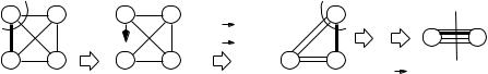
If the graph has too many nodes for the semiexternal algorithm of the preceding subsection, we can try to reduce the number of nodes. This can be done using edge contraction. Suppose we know that e = (u, v) is an MST edge, for example because e is the least-weight edge incident on v. We add e, and somehow need to remember that u and v are already connected in the MST under construction. Above, we used the union–find data structure to record this fact; now we use edge contraction to encode the information into the graph itself. We identify u and v and replace them by a single node. For simplicity, we again call this node u. In other words, we delete v and relink all edges incident on v to u, i.e., any edge (v, w) now becomes an edge (u, w). Figure 11.7 gives an example. In order to keep track of the origin of relinked edges, we associate an additional attribute with each edge that indicates its original endpoints. With this additional information, the MST of the contracted graph is easily translated back to the original graph. We simply replace each edge by its original.
We now have a blueprint for an external MST algorithm: repeatedly find MST edges and contract them. Once the number of nodes is small enough, switch to a semiexternal algorithm. The following subsection gives a particularly simple implementation of this idea.
11.5.3 Sibeyn’s Algorithm
Suppose V = 1..n. Consider the following simple strategy for reducing the number of nodes from n to n [50]:
for v := 1 to n − n do
find the lightest edge (u, v) incident on v and contract it
Figure 11.7 gives an example, with n = 4 and n = 2. The strategy looks deceptively simple. We need to discuss how we find the cheapest edge incident on v and how we relink the other edges incident on v, i.e., how we inform the neighbors of v that they are receiving additional incident edges. We can use a priority queue for both purposes. For each edge e = (u, v), we store the item
(min(u, v), max(u, v), weight of e, origin of e)
a |
7 |
b |
output a |
7 |
|
6 |
9 |
2 |
(a, c) |
9 |
|
3 |
3 |
||||
c |
d |
c |
|||
|
4 |
|
|
4 |
11.5 *External Memory |
227 |
b |
relink |
|
7 |
|
|
) |
|
b |
output (d, b) |
7 |
3 |
|
|
(a, b) |
(c, b) |
|
|
b |
|
|
|
||||
|
|
|
, |
|
|
|
|
|
|
|||
2 |
(a, d) |
(c, d) |
|
a |
|
|
3 |
2 |
... |
c |
d |
|
was |
( |
|
|
|
||||||||
|
|
|
|
|
|
4 |
|
relink |
4 |
9 |
||
d |
|
|
c |
|
|
9 d |
(b, c) (c, d) |
|
||||
|
|
|
|
|
|
|
||||||
|
|
|
|
was |
(a, d) |
|
|
|
||||
Fig. 11.7. An execution of Sibeyn’s algorithm with n = 2. The edge (c, a, 6) is the cheapest edge incident on a. We add it to the MST and merge a into c. The edge (a, b, 7) becomes an edge (c, b, 7) and (a, d, 9) becomes (c, d, 9). In the new graph, (d, b, 2) is the cheapest edge incident on b. We add it to the spanning tree and merge b into d. The edges (b, c, 3) and (b, c, 7) become (d, c, 3) and (d, c, 7), respectively. The resulting graph has two nodes that are connected by four parallel edges of weight 3, 4, 7, and 9, respectively
Function sibeynMST(V, E, c) : Set of Edge
let π be a random permutation of 1..n |
// |
|
|
Q: priority queue |
Order: min node, then min edge weight |
||
foreach e = (u, v) E do |
|
|
|
Q.insert(min {π (u), π (v)}, max {π (u), π (v)}, c(e), u, v)) |
|
||
current := 0 |
|
// we are just before processing node 1 |
|
loop |
|
|
|
(u, v, c, u0, v0) := min Q |
|
// |
next edge |
if current = u then |
|
// new node |
|
if u = n − n + 1 then break loop |
|
// node reduction completed |
|
Q.deleteMin |
|
|
|
output (u0, v0) |
// the original endpoints define an MST edge |
||
(current, relinkTo) := (u, v) |
// |
prepare for relinking remaining u-edges |
|
else if v = relinkTo then |
|
|
|
Q.insert((min {v, relinkTo}, max {v, relinkTo}, c, u0, v0)) |
// relink |
||
S := sort(Q) |
|
// sort by increasing edge weight |
|
apply semiexternal Kruskal to S |
|
|
|
Fig. 11.8. Sibeyn’s MST algorithm
in the priority queue. The ordering is lexicographic by the first and third components, i.e., edges are first ordered by the lower-numbered endpoint and then according to weight. The algorithm operates in phases. In each phase, we select all edges incident on the current node. The lightest edge (= first edge delivered by the queue), say (current, relinkTo), is added to the MST, and all others are relinked. In order to relink an edge (current, z, c, u0, v0) with z = RelinkTo, we add
(min(z, RelinkTo), max(z, RelinkTo), c, u0, v0) to the queue.
Figure 11.8 gives the details. For reasons that will become clear in the analysis, we renumber the nodes randomly before starting the algorithm, i.e., we chose a random permutation of the integers 1 to n and rename node v as π (v). For any edge e = (u, v) we store (min {π (u), π (v)}, max {π (u), π (v)}, c(e), u, v)) in the queue. The main loop stops when the number of nodes is reduced to n . We complete the

228 11 Minimum Spanning Trees
construction of the MST by sorting the remaining edges and then running the semiexternal Kruskal algorithm on them.
Theorem 11.6. Let sort(x) denote the I/O complexity of sorting x items. The expected number of I/O steps needed by the algorithm sibeynMST is O(sort(m ln(n/n ))).
Proof. From Sect. 6.3, we know that an external-memory priority queue can execute K queue operations using O(sort(K)) I/Os. Also, the semiexternal Kruskal step requires O(sort(m)) I/Os. Hence, it suffices to count the number of operations in the reduction phases. Besides the m insertions during initialization, the number of queue operations is proportional to the sum of the degrees of the nodes encountered. Let the random variable Xi denote the degree of node i when it is processed. By the linearity of expectations, we have E[∑1≤i≤n−n Xi] = ∑1≤i≤n−n E[Xi]. The number of edges in the contracted graph is at most m, so that the average degree of a graph with n −i + 1 remaining nodes is at most 2m/(n − i + 1). We obtain.
E ∑ Xi |
= ∑ E[Xi] ≤ |
∑ |
|
2m |
|||||||
n |
− |
i + 1 |
|||||||||
1≤i≤n−n |
1≤i≤n−n |
|
|
|
1≤i≤n−n |
|
|
||||
|
= 2m 1 ∑i |
n |
1 |
− 1 |
∑i n |
|
1 |
= 2m(Hn − Hn ) |
|||
|
i |
|
i |
||||||||
|
≤ ≤ |
|
|
|
≤ ≤ |
|
|
|
|
|
|
= 2m(ln n − ln n ) + O(1) = 2m ln nn + O(1) ,
where Hn := ∑1≤i≤n 1/i = ln n + Θ(1) is the n-th harmonic number (see (A.12)).
Note that we could do without switching to the semiexternal Kruskal algorithm. However, then the logarithmic factor in the I/O complexity would become ln n rather
than ln(n/n ) and the practical performance would be much worse. Observe that n = Θ(M) is a large number, say 108. For n = 1012, ln n is three times ln(n/n ).
Exercise 11.12. For any n, give a graph with n nodes and O(n) edges where Sibeyn’s algorithm without random renumbering would need Ω n2 relink operations.
11.6 Applications
The MST problem is useful in attacking many other graph problems. We shall discuss the Steiner tree problem and the traveling salesman problem.
11.6.1 The Steiner Tree Problem
We are given a nonnegatively weighted undirected graph G = (V, E) and a set S of nodes. The goal is to find a minimum-cost subset T of the edges that connects the nodes in S. Such a T is called a minimum Steiner tree. It is a tree connecting a set U with S U V . The challenge is to choose U so as to minimize the cost of
11.6 Applications |
229 |
the tree. The minimum-spanning-tree problem is the special case where S consists of all nodes. The Steiner tree problem arises naturally in our introductory example. Assume that some of the islands in Taka-Tuka-Land are uninhabited. The goal is to connect all the inhabited islands. The optimal solution will, in general, have some of the uninhabited islands in the solution.
The Steiner tree problem is NP-complete (see Sect. 2.10). We shall show how to construct a solution which is within a factor of two of the optimum. We construct an auxiliary complete graph with node set S: for any pair u and v of nodes in S, the cost of the edge (u, v) in the auxiliary graph is their shortest-path distance in G. Let TA be an MST of the auxiliary graph. We obtain a Steiner tree of G by replacing every edge of TA by the path it represents in G. The resulting subgraph of G may contain cycles. We delete edges from cycles until the remaining subgraph is cycle-free. The cost of the resulting Steiner tree is at most the cost of TA.
Theorem 11.7. The algorithm above constructs a Steiner tree which has at most twice the cost of an optimal Steiner tree.
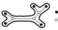
Proof. The algorithm constructs a Steiner tree of cost at most c(TA). It therefore suffices to show that c(TA) ≤ 2c(Topt), where Topt is a minimum Steiner tree for S in G. To this end, it suffices to show that the auxiliary graph has a spanning tree of cost 2c(Topt). Figure 11.9 indicates how to construct such a spanning tree. “Walking once around the Steiner tree” defines a cycle in G of cost 2c(Topt); observe that every edge in Topt occurs exactly twice in this path. Deleting the nodes outside S in this path gives us a cycle in the auxiliary graph. The cost of this path is at most 2c(Topt), because edge costs in the auxiliary graph are shortest-path distances in G. The cycle in the auxiliary graph spans S, and therefore the auxiliary graph has a spanning tree
of cost at most 2c(Topt). |
|
Exercise 11.13. Improve the above bound to 2(1 − 1/|S|) times the optimum. |
|
The algorithm can be implemented to run in time O(m + n log n) [126]. Algorithms with better approximation ratios exist [163].
Exercise 11.14. Outline an implementation of the algorithm above and analyze its running time.
w x
v
node in S
c
node in V \ S
a b
z |
y |
Fig. 11.9. Once around the tree. We have S = {v, w, x, y, z}, and the minimum Steiner tree is shown. The Steiner tree also involves the nodes a, b, and c in V \ S. Walking once around the tree yields the cycle v, a, b, c, w, c, x, c, b, y, b, a, z, a, v . It maps into the cycle v, w, x, y, z, v in the auxiliary graph
230 11 Minimum Spanning Trees
11.6.2 Traveling Salesman Tours
The traveling salesman problem is one of the most intensively studied optimization problems [197, 117, 13]: given an undirected complete graph on a node set V with edge weights c(e), the goal is to find the minimum-weight simple cycle passing through all nodes. This is the path a traveling salesman would want to take whose goal it is to visit all nodes of the graph. We assume in this section that the edge weights satisfy the triangle inequality, i.e., c(u, v) + c(v, w) ≥ c(u, w) for all nodes u, v, and w. There is then always an optimal round trip which visits no node twice (because leaving it out would not increase the cost).
Theorem 11.8. Let Copt and CMST be the cost of an optimal tour and of an MST, respectively. Then
CMST ≤ Copt ≤ 2CMST .
Proof. Let C be an optimal tour. Deleting any edge from C yields a spanning tree. Thus CMST ≤ Copt. Conversely, let T be an MST. Walking once around the tree as shown in Fig. 11.9 gives us a cycle of cost at most 2CMST, passing through all nodes. It may visit nodes several times. Deleting an extra visit to a node does not increase the cost, owing to the triangle inequality.
In the remainder of this section, we shall briefly outline a technique for improving the lower bound of Theorem 11.8. We need two additional concepts: 2-trees and node potentials. Let G be obtained from G by deleting node 1 and the edges incident on it. A minimum 2-tree consists of the two cheapest edges incident on node 1 and an MST of G . Since deleting the two edges incident on node 1 from a tour C yields a spanning tree of G , we have C2 ≤ Copt, where C2 is the minimum cost of a 2-tree. A node potential is any real-valued function π defined on the nodes of G. Any node potential yields a modified cost function cπ by defining
cπ (u, v) = c(u, v) + π (v) + π (u)
for any pair u and v of nodes. For any tour C, the costs under c and cπ differ by 2Sπ := 2 ∑v π (v), since a tour uses exactly two edges incident on any node. Let Tπ be a minimum 2-tree with respect to cπ . Then
cπ (Tπ ) ≤ cπ (Copt) = c(Copt) + 2Sπ ,
and hence
c(Copt) ≥ max (cπ (Tπ ) − 2Sπ ) .
π
This lower bound is known as the Held–Karp lower bound [88, 89]. The maximum is over all node potential functions π . It is hard to compute the lower bound exactly. However, there are fast iterative algorithms for approximating it. The idea is as follows, and we refer the reader to the original papers for details. Assume we have a potential function π and the optimal 2-tree Tπ with respect to it. If all nodes of Tπ have degree two, we have a traveling salesman tour and stop. Otherwise, we make
11.8 Historical Notes and Further Findings |
231 |
the edges incident on nodes of degree larger than two a little more expensive and the edges incident on nodes of degree one a little cheaper. This can be done by modifying the node potential of v as follows. We define a new node potential π by
π (v) = π (v) + ε · (deg(v, Tπ ) − 2)
where ε is a parameter which goes to zero with increasing iteration number, and deg(v, Tπ ) is the degree of v in Tπ . We next compute an optimal 2-tree with respect to π and hope that it will yield a better lower bound.
11.7 Implementation Notes
The minimum-spanning-tree algorithms discussed in this chapter are so fast that the running time is usually dominated by the time required to generate the graphs and appropriate representations. The JP algorithm works well for all m and n if an adjacency array representation (see Sect. 8.2) of the graph is available. Pairing heaps [142] are a robust choice for the priority queue. Kruskal’s algorithm may be faster for sparse graphs, in particular if only a list or array of edges is available or if we know how to sort the edges very efficiently.
The union–find data structure can be implemented more space-efficiently by exploiting the observation that only representatives need a rank, whereas only nonrepresentatives need a parent. We can therefore omit the array rank in Fig. 11.4. Instead, a root of rank g stores the value n + 1 + g in parent. Thus, instead of two arrays, only one array with values in the range 1..n + 1 + log n is needed. This is particularly useful for the semiexternal algorithm.
11.7.1 C++
LEDA [118] uses Kruskal’s algorithm for computing MSTs. The union–find data structure is called partition in LEDA. The Boost graph library [27] gives a choice between Kruskal’s algorithm and the JP algorithm. Boost offers no public access to the union–find data structure.
11.7.2 Java
JDSL [78] uses the JP algorithm.
11.8 Historical Notes and Further Findings
The oldest MST algorithm is based on the cut property and uses edge contractions. Boruvka’s algorithm [28, 148] goes back to 1926 and hence represents one of the oldest graph algorithms. The algorithm operates in phases, and identifies many MST edges in each phase. In a phase, each node identifies the lightest incident edge. These
232 11 Minimum Spanning Trees
edges are added to the MST (here it is assumed that the edge costs are pairwise distinct) and then contracted. Each phase can be implemented to run in time O(m). Since a phase at least halves the number of remaining nodes, only a single node is left after O(log n) phases, and hence the total running time is O(m log n). Boruvka’s algorithm is not often used, because it is somewhat complicated to implement. It is nevertheless important as a basis for parallel MST algorithms.
There is a randomized linear-time MST algorithm that uses phases of Boruvka’s algorithm to reduce the number of nodes [105, 111]. The second building block of this algorithm reduces the number of edges to about 2n: we sample O(m/2) edges randomly, find an MST T of the sample, and remove edges e E that are the heaviest edge in a cycle in e T . The last step is rather difficult to implement efficiently. But, at least for rather dense graphs, this approach can yield a practical improvement [108]. The linear-time algorithm can also be parallelized [84]. An adaptation to the external-memory model [2] saves a factor ln(n/n ) in the asymptotic I/O complexity compared with Sibeyn’s algorithm but is impractical for currently interesting values of n owing to its much larger constant factor in the O-notation.
The theoretically best deterministic MST algorithm [35, 155] has the interesting property that it has optimal worst-case complexity, although it is not exactly known what this complexity is. Hence, if you come up with a completely different deterministic MST algorithm and prove that your algorithm runs in linear time, then we would know that the old algorithm also runs in linear time.
Minimum spanning trees define a single path between any pair of nodes. Interestingly, this path is a bottleneck shortest path [8, Application 13.3], i.e., it minimizes the maximum edge cost for all paths connecting the nodes in the original graph. Hence, finding an MST amounts to solving the all-pairs bottleneck-shortest-path problem in much less time than that for solving the all-pairs shortest-path problem.
A related and even more frequently used application is clustering based on the MST [8, Application 13.5]: by dropping k − 1 edges from the MST, it can be split into k subtrees. The nodes in a subtree T are far away from the other nodes in the sense that all paths to nodes in other subtrees use edges that are at least as heavy as the edges used to cut T out of the MST.
Many applications lead to MST problems on complete graphs. Frequently, these graphs have a compact description, for example if the nodes represent points in the plane and the edge costs are Euclidean distances (these MSTs are called Euclidean minimum spanning trees). In these situations, it is an important concern whether one can rule out most of the edges as too heavy without actually looking at them. This is the case for Euclidean MSTs. It can be shown that Euclidean MSTs are contained in the Delaunay triangulation [46] of the point set. This triangulation has linear size and can be computed in time O(n log n). This leads to an algorithm of the same time complexity for Euclidean MSTs.
We discussed the application of MSTs to the Steiner tree and the traveling salesman problem. We refer the reader to the books [8, 13, 117, 115, 200] for more information about these and related problems.

12
Generic Approaches to Optimization
A smuggler in the mountainous region of Profitania has n items in his cellar. If he sells an item i across the border, he makes a profit pi. However, the smuggler’s trade union only allows him to carry knapsacks with a maximum weight of M. If item i has weight wi, what items should he pack into the knapsack to maximize the profit from his next trip?
This problem, usually called the knapsack problem, has many other applications. The books [122, 109] describe many of them. For example, an investment bank might have an amount M of capital to invest and a set of possible investments. Each investment i has an expected proÞt pi for an investment of cost wi. In this chapter, we use the knapsack problem as an example to illustrate several generic approaches to optimization. These approaches are quite ßexible and can be adapted to complicated situations that are ubiquitous in practical applications.
In the previous chapters we have considered very efÞcient speciÞc solutions for frequently occurring simple problems such as Þnding shortest paths or minimum spanning trees. Now we look at generic solution methods that work for a much larger range of applications. Of course, the generic methods do not usually achieve the same efÞciency as speciÞc solutions. However, they save development time.
Formally, an optimization problem can be described by a set U of potential solutions, a set L of feasible solutions, and an objective function f : L → R. In a maximization problem, we are looking for a feasible solution x L that maximizes the value of the objective function over all feasible solutions. In a minimization problem, we look for a solution that minimizes the value of the objective. In an existence problem, f is arbitrary and the question is whether the set of feasible solutions is nonempty.
For example, in the case of the knapsack problem with n items, a potential solution is simply a vector x = (x1, . . . , xn) with xi {0, 1}. Here xi = 1 indicates that Òelement i is put into the knapsackÓ and xi = 0 indicates that Òelement i is left outÓ. Thus U = {0, 1}n. The proÞts and weights are speciÞed by vectors p = ( p1, . . . , pn) and w = (w1, . . . , wn). A potential solution x is feasible if its weight does not exceed
234 |
12 Generic Approaches to Optimization |
|
|
|||||
|
|
|
Instance |
|
Solutions: |
|
||
|
30 |
|
|
|
|
greedy |
optimal fractional |
|
|
p |
|
|
|
|
3 |
3 |
|
|
20 |
|
|
|
|
|||
|
|
|
|
2 |
|
2 |
||
|
10 |
1 |
2 |
3 |
4 |
1 |
2 |
1 |
|
|
|
|
|
|
|||
|
|
|
2 4 |
w |
|
M = 5 |
5 |
5 |
|
|
|
|
|
||||
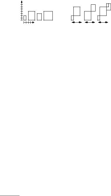
Fig. 12.1. The left part shows a knapsack instance with p = (10, 20, 15, 20), w = (1, 3, 2, 4), and M = 5. The items are indicated as rectangles whose width and height correspond to weight and proÞt, respectively. The right part shows three solutions: the one computed by the greedy algorithm from Sect. 12.2, an optimal solution computed by the dynamic programming algorithm from Sect. 12.3, and the solution of the linear relaxation (Sect. 12.1.1). The optimal solution has weight 5 and proÞt 35
the capacity of the knapsack, i.e., ∑1≤i≤n wixi ≤ M. The dot product w · x is a convenient shorthand for ∑1≤i≤n wixi. We can then say that L = {x U : w · x ≤ M} is the set of feasible solutions and f (x) = p · x is the objective function.
The distinction between minimization and maximization problems is not essential because setting f := − f converts a maximization problem into a minimization problem and vice versa. We shall use maximization as our default simply because our example problem is more naturally viewed as a maximization problem.1
We shall present seven generic approaches. We start out with black-box solvers that can be applied to any problem that can be formulated in the problem speciÞcation language of the solver. In this case, the only task of the user is to formulate the given problem in the language of the black-box solver. Section 12.1 introduces this approach using linear programming and integer linear programming as examples. The greedy approach that we have already seen in Chap. 11 is reviewed in Sect. 12.2. The approach of dynamic programming discussed in Sect. 12.3 is a more ßexible way to construct solutions. We can also systematically explore the entire set of potential solutions, as described in Sect. 12.4. Constraint programming, SAT solvers, and ILP solvers are special cases of systematic search. Finally, we discuss two very ßexible approaches to exploring only a subset of the solution space. Local search, discussed in Sect. 12.5, modiÞes a single solution until it has the desired quality. Evolutionary algorithms, described in Sect. 12.6, simulate a population of candidate solutions.
12.1 Linear Programming – a Black-Box Solver
The easiest way to solve an optimization problem is to write down a speciÞcation of the space of feasible solutions and of the objective function and then use an existing software package to Þnd an optimal solution. Of course, the question is, for what
1 Be aware that most of the literature uses minimization as the default.