Algorithms and data structures

Fig. 4.2. Hashing with linear probing. We have a table t with 13 entries storing synonyms of “(to) hash”. The hash function maps the last character of the word to the integers 0..12 as indicated above the table: a and n are mapped to 0, b and o are mapped to 1, and so on. First, the words are inserted in alphabetical order. Then “clip” is removed. The figure shows the state changes of the table. Gray areas show the range that is scanned between the state changes

of i to check for violations of the invariant. We set j to i + 1. If t[ j] = , we are finished. Otherwise, let f be the element stored in t[ j]. If h( f ) > i, there is nothing to do and we increment j. If h( f ) ≤ i, leaving the hole would violate the invariant, and f would not be found anymore. We therefore move f to t[i] and write into t[ j]. In other words, we swap f and the hole. We set the hole position i to its new position j and continue with j := j + 1. Figure 4.2 gives an example.

Exercise 4.16 (cyclic linear probing). Implement a variant of linear probing, where the table size is m rather than m + m . To avoid overflow at the right-hand end of the array, make probing wrap around. (1) Adapt insert and remove by replacing increments with i := i + 1 mod m. (2) Specify a predicate between(i, j, k) that is true if and only if i is cyclically between j and k. (3) Reformulate the invariant using between.

(4) Adapt remove.

Exercise 4.17 (unbounded linear probing). Implement unbounded hash tables using linear probing and universal hash functions. Pick a new random hash function whenever the table is reallocated. Let α , β , and γ denote constants with 1 < γ < β <

92 4 Hash Tables and Associative Arrays

α that we are free to choose. Keep track of the number of stored elements n. Expand the table to m = β n if n > m/γ . Shrink the table to m = β n if n < m/α . If you do not use cyclic probing as in Exercise 4.16, set m = δ m for some δ < 1 and reallocate the table if the right-hand end should overflow.

4.4 Chaining Versus Linear Probing

We have seen two different approaches to hash tables, chaining and linear probing. Which one is better? This question is beyond theoretical analysis, as the answer depends on the intended use and many technical parameters. We shall therefore discuss some qualitative issues and report on some experiments performed by us.

An advantage of chaining is referential integrity. Subsequent find operations for the same element will return the same location in memory, and hence references to the results of find operations can be established. In contrast, linear probing moves elements during element removal and hence invalidates references to them.

An advantage of linear probing is that each table access touches a contiguous piece of memory. The memory subsystems of modern processors are optimized for this kind of access pattern, whereas they are quite slow at chasing pointers when the data does not fit into cache memory. A disadvantage of linear probing is that search times become high when the number of elements approaches the table size. For chaining, the expected access time remains small. On the other hand, chaining wastes space on pointers that linear probing could use for a larger table. A fair comparison must be based on space consumption and not just on table size.

We have implemented both approaches and performed extensive experiments. The outcome was that both techniques performed almost equally well when they were given the same amount of memory. The differences were so small that details of the implementation, compiler, operating system, and machine used could reverse the picture. Hence we do not report exact figures.

However, we found chaining harder to implement. Only the optimizations discussed in Sect. 4.6 made it competitive with linear probing. Chaining is much slower if the implementation is sloppy or memory management is not implemented well.

4.5 *Perfect Hashing

The hashing schemes discussed so far guarantee only expected constant time for the operations find, insert, and remove. This makes them unsuitable for real-time applications that require a worst-case guarantee. In this section, we shall study perfect hashing, which guarantees constant worst-case time for find. To keep things simple, we shall restrict ourselves to the static case, where we consider a fixed set S of n elements with keys k1 to kn.

In this section, we use Hm to denote a family of c-universal hash functions with range 0..m − 1. In Exercise 4.11, it is shown that 2-universal classes exist for every

m. For h Hm, we use C(h) to denote the number of collisions produced by h, i.e., the number of pairs of distinct keys in S which are mapped to the same position:

C(h) = {(x, y) : x, y S, x = y and h(x) = h(y)} .

As a first step, we derive a bound on the expectation of C(h).

Lemma 4.5. E[C(h)] ≤ cn(n − 1)/m. Also, for at least half of the functions h Hm, we have C(h) ≤ 2cn(n −1)/m.

Proof. We define n(n −1) indicator random variables Xi j(h). For i = j, let Xi j(h) = 1 iff h(ki) = h(k j). Then C(h) = ∑i j Xi j(h), and hence

E[C] = E[∑Xi j] = ∑E[Xi j] = ∑prob(Xi j = 1) ≤ n(n −1) · c/m ,

i j i j i j

where the second equality follows from the linearity of expectations (see (A.2)) and the last equality follows from the universality of Hm. The second claim follows from Markov’s inequality (A.4).

If we are willing to work with a quadratic-size table, our problem is solved.

Lemma 4.6. If m ≥ cn(n − 1) + 1, at least half of the functions h Hm operate injectively on S.

Proof. By Lemma 4.5, we have C(h) < 2 for half of the functions in Hm. Since C(h) is even, C(h) < 2 implies C(h) = 0, and so h operates injectively on S.

So we choose a random h Hm with m ≥ cn(n − 1) + 1 and check whether it is injective on S. If not, we repeat the exercise. After an average of two trials, we are successful.

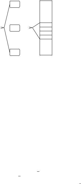
In the remainder of this section, we show how to bring the table size down to linear. The idea is to use a two-stage mapping of keys (see Fig. 4.3). The first stage maps keys to buckets of constant average size. The second stage uses a quadratic amount of space for each bucket. We use the information about C(h) to bound the number of keys hashing to any table location. For 0..m −1 and h Hm, let Bh be the elements in S that are mapped to by h and let bh be the cardinality of Bh.

Lemma 4.7. C(h) = ∑ bh(bh −1).

Proof. For any , the keys in Bh give rise to bh(bh − 1) pairs of keys mapping to the same location. Summation over completes the proof.

The construction of the perfect hash function is now as follows. Let α be a constant, which we shall fix later. We choose a hash function h H α n to split S into subsets B . Of course, we choose h to be in the good half of H α n , i.e., we choose

h H α n with C(h) ≤ 2cn(n −1)/ α n ≤ 2cn/α . For each , let B be the elements in S mapped to and let b = |B |.

94 4 Hash Tables and Associative Arrays

Fig. 4.3. Perfect hashing. The top-level hash function h splits S into subsets B0, . . . , B , . . . .

Let b = |B | and m = cb (b − 1) + 1. The function h maps B injectively into a table of size m . We arrange the subtables into a single table. The subtable for B then starts at position s = m0 + . . . + m −1 and ends at position s + m −1

Now consider any B . Let m = cb (b − 1) + 1. We choose a function h Hm which maps B injectively into 0..m − 1. Half of the functions in Hm have this property by Lemma 4.6 applied to B . In other words, h maps B injectively into a table of size m . We stack the various tables on top of each other to obtain one large table of size ∑ m . In this large table, the subtable for B starts at position s = m0 + m1 + . . . + m −1. Then

:= h(x); return s + h (x)

computes an injective function on S. This function is bounded by

∑m ≤ α n + c · ∑b (b −1)

≤1 + α n + c ·C(h)

≤1 + α n + c · 2cn/α

≤1 + (α + 2c2/α )n ,

and hence we have constructed a perfect hash function that maps S into a linearly sized range, namely 0..(α + 2c2/α )n. In the derivation above, the first inequality

uses the definition of the m ’s, the second inequality uses Lemma 4.7, and the third

√

inequality uses C(h) ≤ 2cn/α . The choice α = 2c minimizes the size of the range.

√

For c = 1, the size of the range is 2 2n.

√

Theorem 4.8. For any set of n keys, a perfect hash function with range 0..2 2n can be constructed in linear expected time.

Constructions with smaller ranges are known. Also, it is possible to support insertions and deletions.

Exercise 4.18 (dynamization). We outline a scheme for “dynamization” here. Consider a fixed S, and choose h H2 α n . For any , let m = 2cb (b − 1) + 1, i.e., all m’s are chosen to be twice as large as in the static scheme. Construct a perfect hash function as above. Insertion of a new x is handled as follows. Assume that h maps x onto . If h is no longer injective, choose a new h . If b becomes so large that m = cb (b −1) + 1, choose a new h.

4.6 Implementation Notes

Although hashing is an algorithmically simple concept, a clean, efficient, robust implementation can be surprisingly nontrivial. Less surprisingly, the hash functions are the most important issue. Most applications seem to use simple, very fast hash functions based on exclusive-OR, shifting, and table lookup rather than universal hash functions; see, for example, www.burtleburtle.net/bob/hash/doobs.html or search for “hash table” on the Internet. Although these functions seem to work well in practice, we believe that the universal families of hash functions described in Sect. 4.2 are competitive. Unfortunately, there is no implementation study covering all of the fastest families. Thorup [191] implemented a fast family with additional properties. In particular, the family H [] considered in Exercise 4.15 should be suitable for integer keys, and Exercise 4.8 formulates a good function for strings. It might be possible to implement the latter function to run particularly fast using the SIMD instructions of modern processors that allow the parallel execution of several operations.

Hashing with chaining uses only very specialized operations on sequences, for which singly linked lists are ideally suited. Since these lists are extremely short, some deviations from the implementation scheme described in Sect. 3.1 are in order. In particular, it would be wasteful to store a dummy item with each list. Instead, one should use a single shared dummy item to mark the ends of all lists. This item can then be used as a sentinel element for find and remove, as in the function findNext in Sect. 3.1.1. This trick not only saves space, but also makes it likely that the dummy item will reside in the cache memory.

With respect to the first element of the lists, there are two alternatives. One can either use a table of pointers and store the first element outside the table, or store the first element of each list directly in the table. We refer to these alternatives as slim tables and fat tables, respectively. Fat tables are usually faster and more spaceefficient. Slim tables are superior when the elements are very large. Observe that a slim table wastes the space occupied by m pointers and that a fat table wastes the space of the unoccupied table positions (see Exercise 4.6). Slim tables also have the advantage of referential integrity even when tables are reallocated. We have already observed this complication for unbounded arrays in Sect. 3.6.

Comparing the space consumption of hashing with chaining and hashing with linear probing is even more subtle than is outlined in Sect. 4.4. On the one hand, linked lists burden the memory management with many small pieces of allocated memory; see Sect. 3.1.1 for a discussion of memory management for linked lists.

96 4 Hash Tables and Associative Arrays

On the other hand, implementations of unbounded hash tables based on chaining can avoid occupying two tables during reallocation by using the following method. First, concatenate all lists into a single list L. Deallocate the old table. Only then, allocate the new table. Finally, scan L, moving the elements to the new table.

Exercise 4.19. Implement hashing with chaining and hashing with linear probing on your own machine using your favorite programming language. Compare their performance experimentally. Also, compare your implementations with hash tables available in software libraries. Use elements of size eight bytes.

Exercise 4.20 (large elements). Repeat the above measurements with element sizes of 32 and 128. Also, add an implementation of slim chaining, where table entries only store pointers to the first list element.

Exercise 4.21 (large keys). Discuss the impact of large keys on the relative merits of chaining versus linear probing. Which variant will profit? Why?

Exercise 4.22. Implement a hash table data type for very large tables stored in a file. Should you use chaining or linear probing? Why?

4.6.1 C++

The C++ standard library does not (yet) define a hash table data type. However, the popular implementation by SGI (http://www.sgi.com/tech/stl/) offers several variants: hash_set, hash_map, hash_multiset, and hash_multimap.7 Here “set” stands for the kind of interface used in this chapter, whereas a “map” is an associative array indexed by keys. The prefix “multi” indicates data types that allow multiple elements with the same key. Hash functions are implemented as function objects, i.e., the class hash<T> overloads the operator “()” so that an object can be used like a function. The reason for this approach is that it allows the hash function to store internal state such as random coefficients.

LEDA [118] offers several hashing-based implementations of dictionaries. The class h_array Key, T offers associative arrays for storing objects of type T . This class requires a user-defined hash function int Hash(Key&) that returns an integer value which is then mapped to a table index by LEDA. The implementation uses hashing with chaining and adapts the table size to the number of elements stored. The class map is similar but uses a built-in hash function.

Exercise 4.23 (associative arrays). Implement a C++ class for associative arrays. Support operator[] for any index type that supports a hash function. Make sure that H[x]=... works as expected if x is the key of a new element.

4.6.2 Java

The class java.util.HashMap implements unbounded hash tables using the function hashCode defined in the class Object as a hash function.

7Future versions of the standard will have these data types using the word “unordered” instead of the word “hash”.

4.7 Historical Notes and Further Findings

Hashing with chaining and hashing with linear probing were used as early as the 1950s [153]. The analysis of hashing began soon after. In the 1960s and 1970s, average-case analysis in the spirit of Theorem 4.1 and Exercise 4.7 prevailed. Various schemes for random sets of keys or random hash functions were analyzed. An early survey paper was written by Morris [143]. The book [112] contains a wealth of material. For example, it analyzes linear probing assuming random hash functions. Let n denote the number of elements stored, let m denote the size of the table and set α = n/m. The expected number Tfail of table accesses for an unsuccessful search and the number Tsuccess for a successful search are about

respectively. Note that these numbers become very large when n approaches m, i.e., it is not a good idea to fill a linear-probing table almost completely.

Universal hash functions were introduced by Carter and Wegman [34]. The original paper proved Theorem 4.3 and introduced the universal classes discussed in Exercise 4.11. More on universal hashing can be found in [10].

Perfect hashing was a black art until Fredman, Komlos, and Szemeredi [66] introduced the construction shown in Theorem 4.8. Dynamization is due to Dietzfelbinger et al. [54]. Cuckoo hashing [152] is an alternative approach to perfect hashing.

A minimal perfect hash function bijectively maps a set S 0..U −1 to the range 0..n − 1, where n = |S|. The art is to do this in constant time and with very little space – Ω(n) bits is a lower bound. There are now practicable schemes that achieve this bound [29]. One variant assumes three truly random hash functions8 hi : 0..U − 1 → im/3..(i + 1)m/3 − 1 for i 0..2 and m ≈ 1.23n. In a first mapping step, a key k 0..U −1 is mapped to

p(k) = hi(k), where i = g(h0(k)) g(h1(k)) g(h2(k)) mod 3 ,

and g : 0..α n → {0, 1, 2} is a lookup table that is precomputed using some simple greedy algorithm. In a second ranking step, the set 0..α n is mapped to 0..n − 1, i.e., h(k) = rank( p(k)), where rank(i) = |{k S : p(k) ≤ i}|. This ranking problem is a standard problem in the field of succinct data structures and can be supported in constant time using O(n) bits of space.

Universal hashing bounds the probability of any two keys colliding. A more general notion is k-way independence, where k is a positive integer. A family H of hash

functions is k-way independent if for some constant c, any k distinct keys x1 to xk, and any k hash values a1 to ak, prob(h(x1) = a1 ··· h(xk) = ak) ≤ c/mk. The polynomials of degree k − 1 with random coefficients are a simple k-wise independent

family of hash functions [34] (see Exercise 4.12).

8Actually implementing such hash functions would require Ω(n log n) bits. However, this problem can be circumvented by first splitting S into many small buckets. We can then use the same set of fully random hash functions for all the buckets [55].

98 4 Hash Tables and Associative Arrays

Cryptographic hash functions need stronger properties than what we need for

hash tables. Roughly, for a value x, it should be difficult to come up with a value x such that h(x ) = h(x).

5

Sorting and Selection

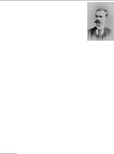
Telephone directories are sorted alphabetically by last name. Why? Because a sorted index can be searched quickly. Even in the telephone directory of a huge city, one can usually find a name in a few seconds. In an unsorted index, nobody would even try to find a name. To a first approximation, this chapter teaches you how to turn an unordered collection of elements into an ordered collection, i.e., how to sort the collection. However, sorting has many other uses as well. An early example of a massive data-processing task was the statistical evaluation of census data; 1500 people needed seven years to manually process data from the US census in 1880. The engineer Herman Hollerith,1 who participated in this evaluation as a statistician, spent much of the ten years to the next census developing counting and sorting machines for mechanizing this gigantic endeavor. Although the 1890 census had to evaluate more people and more questions, the basic evaluation was finished in 1891. Hollerith’s company continued to play an important role in the development of the information-processing industry; since 1924, it has been known as International Business Machines (IBM). Sorting is important for census statistics because one often wants to form subcollections, for example, all persons between age 20 and 30 and living on a farm. Two applications of sorting solve the problem. First, we sort all persons by age and form the subcollection of persons between 20 and 30 years of age. Then we sort the subcollection by home and extract the subcollection of persons living on a farm.

Although we probably all have an intuitive concept of what sorting is about, let us give a formal deÞnition. The input is a sequence s = e1, . . . , en of n elements. Each element ei has an associated key ki = key(ei). The keys come from an ordered universe, i.e., there is a linear order ≤ deÞned on the keys.2 For ease of notation, we extend the comparison relation to elements so that e ≤ e if and only

1The photograph was taken by C. M. Bell (see US Library of CongressÕs Prints and Photographs Division, ID cph.3c15982).

2A linear order is a reßexive, transitive, and weakly antisymmetric relation. In contrast to a total order, it allows equivalent elements (see Appendix A for details).

100 5 Sorting and Selection

if key(e) ≤ key(e ). The task is to produce a sequence s = e1, . . . , en such that s is a permutation of s and such that e1 ≤ e2 ≤ ··· ≤ en. Observe that the ordering of equivalent elements is arbitrary.

Although different comparison relations for the same data type may make sense, the most frequent relations are the obvious order for numbers and the lexicographic order (see Appendix A) for tuples, strings, and sequences. The lexicographic order for strings comes in different ßavors. We may treat corresponding lower-case and upper-case characters as being equivalent, and different rules for treating accented characters are used in different contexts.

Exercise 5.1. Given linear orders ≤A for A and ≤B for B, deÞne a linear order on

A × B.

Exercise 5.2. DeÞne a total order for complex numbers with the property that x ≤ y implies |x| ≤ |y|.

Sorting is a ubiquitous algorithmic tool; it is frequently used as a preprocessing step in more complex algorithms. We shall give some examples.

•Preprocessing for fast search. In Sect. 2.5 on binary search, we have already seen that a sorted directory is easier to search, both for humans and computers. Moreover, a sorted directory supports additional operations, such as Þnding all elements in a certain range. We shall discuss searching in more detail in Chap. 7. Hashing is a method for searching unordered sets.

•Grouping. Often, we want to bring equal elements together to count them, eliminate duplicates, or otherwise process them. Again, hashing is an alternative. But sorting has advantages, since we shall see rather fast, space-efÞcient, deterministic sorting algorithm that scale to huge data sets.

•Processing in a sorted order. Certain algorithms become very simple if the inputs are processed in sorted order. Exercise 5.3 gives an example. Other examples are KruskalÕs algorithm in Sect. 11.3 and several of the algorithms for the knapsack problem in Chap. 12. You may also want to remember sorting when you solve Exercise 8.6 on interval graphs.

In Sect. 5.1, we shall introduce several simple sorting algorithms. They have quadratic complexity, but are still useful for small input sizes. Moreover, we shall learn some low-level optimizations. Section 5.2 introduces mergesort, a simple divide-and-conquer sorting algorithm that runs in time O(n log n). Section 5.3 establishes that this bound is optimal for all comparison-based algorithms, i.e., algorithms that treat elements as black boxes that can only be compared and moved around. The quicksort algorithm described in Sect. 5.4 is again based on the divide-and-conquer principle and is perhaps the most frequently used sorting algorithm. Quicksort is also a good example of a randomized algorithm. The idea behind quicksort leads to a simple algorithm for a problem related to sorting. Section 5.5 explains how the k-th smallest of n elements can be selected in time O(n). Sorting can be made even faster than the lower bound obtained in Sect. 5.3 by looking at the bit patterns of the keys, as explained in Sect. 5.6. Finally, Section 5.7 generalizes quicksort and mergesort to very good algorithms for sorting inputs that do not Þt into internal memory.