

Molecular Fluorescence
.pdf6.1 Steady-state spectrofluorometry 165
As previously outlined, the emission correction factors must be recorded with an emission polarizer in a defined orientation (preferably at the magic angle), and this orientation must be kept unchanged for recording emission or excitation spectra irrespective of whether or not the fluorescence is polarized.
6.1.6
Measurement of steady-state emission anisotropy. Polarization spectra
Let us recall the definition of the emission anisotropy r (see Chapter 5) in a configuration where the exciting light is vertically polarized and the emitted fluorescence is observed at right angles in a horizontal plane (Figure 6.4):
Ik I? |
|
r ¼ Ik þ 2I? |
ð6:6Þ |
where Ik and I? are the polarized components parallel and perpendicular to the direction of polarization of the incident light, respectively.
r can be determined with a spectrofluorometer equipped with polarizers. It is not su cient to keep the excitation polarizer vertical and to rotate the emission polarizer because, as already mentioned, the transmission e ciency of a monochromator depends on the polarization of the light. The determination of the emission anisotropy requires four intensity measurements: IVV; IVH; IHV and IHH (V: vertical; H: horizontal; the first subscript corresponds to the orientation of the excitation polarizer and the second subscript to the emission polarizer) (Figure 6.4).
For a horizontally polarized exciting light, the vertical component ðIHVÞ and the horizontal component ðIHHÞ of the fluorescence detected through the emission monochromator are di erent, although these components are identical before entering the monochromator according to the Curie symmetry principle (see Chapter 5). The G factor6), G ¼ IHV=IHH, measured through the monochromator, varies from 1 and can be used as a correcting factor for the ratio Ik=I? because it represents the ratio of the sensitivities of the detection system for vertically and horizontally polarized light:
IVV ¼ G Ik
IVH I?
Equation (6.6) then becomes
r ¼ IVV GIVH
IVV þ 2GIVH
6)The letter G comes from ‘grating’. In fact, the majority of the polarization e ects arise from the polarization dependence of the monochromator grating, but the detector response and the optics can contribute to a lesser extent.
ð6:7Þ
ð6:8Þ7)
7)For the sake of simplicity, this relation is often written as
r ¼ Ik GI? Ik þ 2GI?

166 6 Principles of steady-state and time-resolved fluorometric techniques
Fig. 6.4. Schematic diagram showing how the four intensity components are measured for determination of the steady-state anisotropy.
The excitation polarization spectrum (which represents the variation of r as a function of the excitation wavelength; see Chapter 5) is obtained by recording the variations of IVVðlEÞ, IVHðlEÞ, IHVðlEÞ, and IHHðlEÞ and by calculating rðlEÞ by means of Eq. (6.8) with GðlEÞ ¼ IVHðlEÞ=IHHðlEÞ. The correction factors for wavelength dependence can be ignored because they cancel out in the ratio.

6.2 Time-resolved fluorometry 167
In some cases, filters are used instead of the emission monochromator. In principle, no G factor is then considered, but in practice, e ects may be due to the sensitivity of the photomultipliers to polarization (in particular, photomultipliers with side-on photocathodes).
6.2
Time-resolved fluorometry
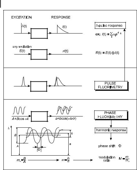
Knowledge of the dynamics of excited states is of major importance in understanding photophysical, photochemical and photobiological processes. Two time-resolved techniques, pulse fluorometry and phase-modulation fluorometry, are commonly used to recover the lifetimes, or more generally the parameters characterizing the d-pulse response of a fluorescent sample (i.e. the response to an infinitely short pulse of light expressed as the Dirac function d).
Pulse fluorometry uses a short exciting pulse of light and gives the d-pulse response of the sample, convoluted by the instrument response. Phase-modulation fluorometry uses modulated light at variable frequency and gives the harmonic response of the sample, which is the Fourier transform of the d-pulse response. The first technique works in the time domain, and the second in the frequency domain. Pulse fluorometry and phase-modulation fluorometry are theoretically equivalent, but the principles of the instruments are di erent. Each technique will now be presented and then compared.
6.2.1
General principles of pulse and phase-modulation fluorometries
The principles of pulse and phase-modulation fluorometries are illustrated in Figures 6.5 and 6.6. The d-pulse response IðtÞ of the fluorescent sample is, in the simplest case, a single exponential whose time constant is the excited-state lifetime, but more often it is a sum of discrete exponentials, or a more complicated function; sometimes the system is characterized by a distribution of decay times. For any excitation function EðtÞ, the response RðtÞ of the sample is the convolution product of this function by the d-pulse response:
t |
|
RðtÞ ¼ EðtÞ nIðtÞ ¼ ð y Eðt0ÞIðt t0Þ dt0 |
ð6:9Þ8) |
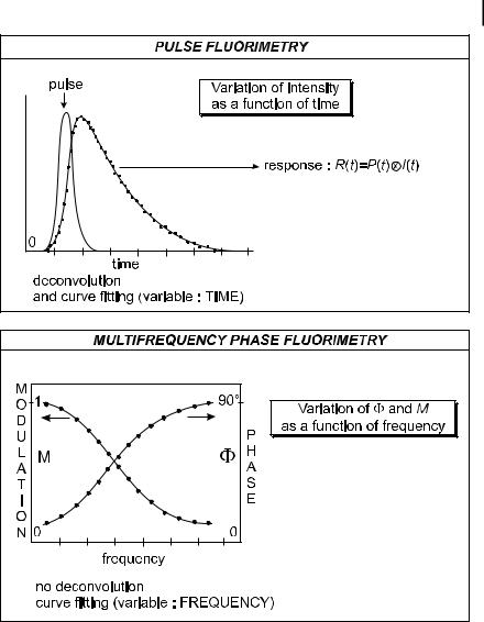
Pulse fluorometry The sample is excited by a short pulse of light and the fluorescence response is recorded as a function of time. If the duration of the pulse is long
8)The convolution integral appearing in this equation can be easily understood by considering the excitation function as successive Dirac functions at various times t.
168 6 Principles of steady-state and time-resolved fluorometric techniques
Fig. 6.5. Principles of time-resolved fluorometry.
with respect to the time constants of the fluorescence decay, the fluorescence response is the convolution product given by Eq. (6.9): the fluorescence intensity increases, goes through a maximum and becomes identical to the true d-pulse response iðtÞ as soon as the intensity of the light pulse is negligible (Figure 6.6). In this case, data analysis for the determination of the parameters characterizing the d-pulse response requires a deconvolution of the fluorescence response (see Section 6.2.5).
Phase-modulation fluorometry The sample is excited by a sinusoidally modulated light at high frequency. The fluorescence response, which is the convolution product (Eq. 6.9) of the d-pulse response by the sinusoidal excitation function, is sinusoidally
6.2 Time-resolved fluorometry 169
Fig. 6.6. Principles of pulse fluorometry and multi-frequency phase-modulation fluorometry.
modulated at the same frequency but delayed in phase and partially demodulated with respect to the excitation. The phase shift F and the modulation ratio M (equal to m=m0), i.e. the ratio of the modulation depth m (AC/DC ratio) of the fluorescence and the modulation depth of the excitation m0; see Figure 6.5) characterize the harmonic response of the system. These parameters are measured as a function of the modulation frequency. No deconvolution is necessary because the data are directly analyzed in the frequency domain (Figure 6.6).
170 |
6 Principles of steady-state and time-resolved fluorometric techniques |
|
|
Relationship between harmonic response and d-pulse response |
It is worth demon- |
|
||
|
strating that the harmonic response is the Fourier transform of the d-pulse response. |
|
|
The sinusoidal excitation function can be written as |
|
|
EðtÞ ¼ E0½1 þ m0 expðjotÞ& |
ð6:10Þ9) |
where o is the angular frequency ð¼ 2p f Þ. The response of the system is calculated using Eq. (6.9), which gives, after introducing the new variable u ¼ t t0
|
y |
y |
IðuÞ expð jouÞ du |
|
RðtÞ ¼ E0 |
ð0 |
IðuÞ du þ m0 expðjotÞ ð0 |
ð6:11Þ |
It is convenient for the calculations to use the normalized d-pulse response iðtÞ according to
ðy
iðtÞ dt ¼ 1 |
ð6:12Þ |
0
The fluorescence response can then be written:
RðtÞ ¼ E0½1 þ m expðjot FÞ& |
ð6:13Þ |
||
with |
|
|
|
|
y |
|
|
m expð jFÞ ¼ m0 |
ð0 |
iðuÞ expð jouÞ du |
ð6:14Þ |
Using the modulation ratio M ¼ m=m0 and replacing u by t for clarity, we obtain
|
y |
|
|
|
|
M expð jFÞ ¼ ð0 |
iðtÞ expð jotÞ dt |
|
ð6:15Þ |
This important expression shows that the harmonic response |
expressed as |
|||
M expð jFÞ is the Fourier transform of the d-pulse response. |
|
|||
It is convenient to introduce the sine and cosine transforms P and Q of the d- pulse response:
y |
|
|
P ¼ ð0 |
iðtÞ sinðotÞ dt |
ð6:16Þ |
y |
|
|
Q ¼ ð0 |
iðtÞ cosðotÞ dt |
ð6:17Þ |
9) expð jotÞ ¼ cosðotÞ þ j sinðotÞ

6.2 Time-resolved fluorometry 171
If the d-pulse response is not normalized according to Eq. (6.12), then Eqs (6.16) and (6.17) should be replaced by
|
|
y I t |
sin ot |
dt |
|
|
|
|||||
|
P ¼ |
Ð0 |
ð0yÞ I t ðdt Þ |
|
|
|
ð6:18Þ |
|||||
|
|
|
Ð |
|
ð Þ |
|
|
|
|
|
|
|
|
|
|
|
|
|
|
|
|
|
|
|
|
|
|
y I |
t |
cos ot dt |
|
|
||||||
|
Q ¼ |
Ð0 |
ð0yÞ I t ðdt Þ |
|
|
ð6:19Þ |
||||||
|
|
|
Ð |
|
ð Þ |
|
|
|
|
|
|
|
Equation (6.15) can be rewritten as |
|
|||||||||||
|
M cos F jM sin F ¼ Q jP |
ð6:20Þ |
||||||||||
Therefore, |
|
|
|
|
|
|
|
|
|
|
||
|
M sin F ¼ P |
|
|
|
|
|
|
|
ð6:21Þ |
|||
|
M cos F ¼ Q |
|
|
|
|
|
|
|
ð6:22Þ |
|||
Appropriate combinations of these two equations lead to |
|
|||||||||||
|
|
|
|
|
|
|
|
|
|
|
|
|
|
|
|
|
|
P |
|
|
|
|
|
|
|
|
F ¼ tan 1 |
|
|
|
|
|
|
|
|
ð6:23Þ |
||
|
Q |
|
|
|
|
|
||||||
|
|
|
|
|
|
|
|
|
||||
|
M ¼ ½P2 þ Q 2&1=2 |
|
|
|
|
ð6:24Þ |
||||||
In practice, the phase shift F and the modulation ratio M are measured as a function of o. Curve fitting of the relevant plots (Figure 6.6) is performed using the theoretical expressions of the sine and cosine Fourier transforms of the d-pulse response and Eqs (6.23) and (6.24). In contrast to pulse fluorometry, no deconvolution is required.
General relations for single exponential and multi-exponential decays For a single exponential decay, the d-pulse response is
|
IðtÞ ¼ a expð t=tÞ |
|
|
ð6:25Þ |
|||
where t is the decay time and a is the pre-exponential factor or amplitude. |
|
||||||
|
The phase shift and relative modulation are related to the decay time by |
|
|||||
|
|
|
|
|
|
|
|
|
tan F ¼ ot |
|
|
|
ð6:26Þ |
||
|
|
|
|
|
|
|
|
|
1 |
|
|
|
|
|
|
|
M ¼ |
|
|
|
ð6:27Þ |
||
|
ð1 þ o2t2Þ1=2 |
|
|||||

172 6 Principles of steady-state and time-resolved fluorometric techniques
For a multi-exponential decay with n components, the d-pulse response is
Xn
IðtÞ ¼ |
ai expð t=tiÞ |
ð6:28Þ |
|
i¼1 |
|
Note that the fractional intensity of component i, i.e. the fractional contribution of component i to the total steady-state intensity is
|
y Ii t |
dt |
|
aiti |
|
||
|
0 |
|
|
|
|
|
|
fi ¼ |
Ð0y I |
ðt |
Þdt |
¼ |
|
|
ð6:29Þ |
n |
|
||||||
|
Ð |
ð Þ |
|
i¼1 aiti |
|
||
|
|
|
|
n |
P |
|
|
|
|
|
|
|
¼ 1. |
|
|
with, of course, P fi |
|
||||||
i¼1
Using Eqs (6.18) and (6.19), the sine and cosine Fourier transforms, P and Q , are given by
|
|
n |
|
|
aiti2 |
|
|
|
|
|
|
|
|
|
|
|||
|
|
o |
|
|
|
|
|
|
|
|
|
|
n |
|
|
|
|
|
|
|
|
1 |
|
|
o |
2t2 |
|
|
|
fi ti |
|
|
|
||||
|
|
i¼1 |
|
|
|
|
|
|
|
|
||||||||
|
|
|
|
|
|
|
|
|
|
|
||||||||
|
|
|
|
|
|
|
i |
|
|
|
|
|
|
|
|
|
||
P |
¼ |
Pn |
þ |
|
|
|
¼ |
o |
|
|
|
|
ð |
6:30 |
||||
|
|
|
|
aiti |
|
|
|
|
i 1 1 þ o |
ti |
Þ |
|||||||
|
|
|
|
|
|
|
|
|
|
|
|
|
¼ |
|
|
|
|
|
|
|
|
i¼1 |
|
|
|
|
|
|
|
X |
|
|
|
|
|
||
|
|
n |
P |
aiti |
|
|
|
|
|
|
|
|
|
|
|
|||
|
|
|
|
|
|
|
|
|
|
|
|
|
|
|
||||
|
|
|
|
|
|
|
|
|
|
|
|
|
|
|
|
|||
|
|
i¼1 |
1 |
|
|
o2t2 |
|
|
n |
|
fi |
|
|
|
|
|||
|
|
|
|
|
|
|
|
|
|
|
|
|
||||||
Q |
¼ |
P nþ |
|
|
|
¼ i |
|
|
2 |
2 |
|
ð |
6:31 |
|||||
|
|
|
|
aiti |
|
1 1 þ o |
ti |
|
Þ |
|||||||||
|
|
|
|
|
|
|
|
|
|
|
¼ |
|
|
|
|
|
|
|
|
|
|
|
|
|
|
|
|
|
X |
|
|
|
|
|
|
||
P
i¼1
These equations are to be used in conjunction with Eqs (6.23) and (6.24) giving F and M.
When the fluorescence decay of a fluorophore is multi-exponential, the natural way of defining an average decay time (or lifetime) is:
|
|
|
|
y tI t dt |
0y t |
n |
ai expð t=tiÞ dt |
|
|||||
hti |
|
¼ |
0 |
|
ð Þ |
|
¼ Ð y |
|
i¼1 |
|
|
||
|
|
|
I t dt |
|
|
|
|||||||
|
f |
Ð |
0 |
|
|
P |
|
|
|||||
|
|
|
Ð |
|
|
ð Þ |
|
0 |
i¼1 ai expð t=tiÞ dt |
Þ |
|||
|
|
|
n |
|
|
|
|
Ð |
P |
ð |
|||
|
|
|
|
¼ |
|
|
6:32 |
||||||
|
|
¼ P |
|
|
|
|
|
|
|
||||
|
|
|
i¼1 |
aiti2 |
n |
|
|
|
|
||||
|
|
|
|
|
X |
|
|
|
|
||||
htif |
|
n |
|
|
|
|
fi ti |
|
|
|
|
||
|
|
|
P |
|
aiti |
i¼1 |
|
|
|
|
|||
|
|
|
|
|
|
|
|
|
|
||||
i¼1
In this definition, each decay time is weighted by the corresponding fractional intensity. This average is called the intensity-averaged decay time (or lifetime).
Another possibility is to use the amplitudes (pre-exponential factors) as weights:
|
|
n |
|
|
|
|
|
|
aiti |
|
n |
|
|
|
|
i¼1 |
|
X |
|
|
htia |
¼ |
P |
¼ |
aiti |
ð |
Þ |
|
n |
|
|
6:33 |
||
|
|
P |
|
i¼1 |
|
|
|
|
ai |
|
|
|
|
|
|
i¼1 |
|
|
|
|

173
where ai are the fractional amplitudes
ai
ai ¼ Pn
ai
i¼1
Pn
with, of course, (or lifetime). i¼1
The definition used depends on the phenomenon under study. For instance, the intensity-averaged lifetime must be used for the calculation of an average collisional quenching constant, whereas in resonance energy transfer experiments, the amplitude-averaged decay time or lifetime must be used for the calculation of energy transfer e ciency (see Section 9.2.1).
6.2.2
Design of pulse fluorometers
6.2.2.1 Single-photon timing technique
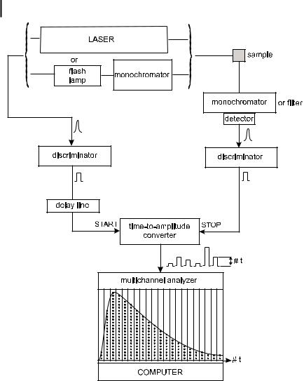
Pulse fluorometry is the most popular technique for the determination of lifetimes (or decay parameters). Most instruments are based on the time-correlated singlephoton counting (TCSPC) method, better called as single-photon timing (SPT). The basic principle relies on the fact that the probability of detecting a single photon at time t after an exciting pulse is proportional to the fluorescence intensity at that time. After timing and recording the single photons following a large number of exciting pulses, the fluorescence intensity decay curve is reconstructed.
Figure 6.7 shows a conventional single-photon counting instrument. The excitation source can be either a flash lamp or a mode-locked laser. An electrical pulse associated with the optical pulse is generated (e.g. by a photodiode or the electronics associated with the excitation source) and routed – through a discriminator – to the start input of the time-to-amplitude converter (TAC). Meanwhile, the sample is excited by the optical pulse and emits fluorescence. The optics are tuned (e.g. by means of a neutral density filter) so that the photomultiplier detects no more than one photon for each exciting pulse. The corresponding electrical pulse is routed – through a discriminator – to the stop input of the TAC. The latter generates an output pulse whose amplitude is directly proportional to the delay time between the start and the stop pulses10). The height analysis of this pulse is achieved by an analogue-to-digital converter and a multichannel analyzer (MCA), which increases by one the contents of the memory channel corresponding to the digital value of the pulse. After a large number of excitation and detection events, the histogram of pulse heights represents the fluorescence decay curve. Obviously, the larger the number of events, the better the accuracy of the decay curve. The required accuracy
10)The start pulse initiates charging of a capacitor and the stop pulse stops the charging ramp. The pulse delivered by the
TAC is proportional to the final voltage of the capacitor, i.e. proportional to the delay time between the start and the stop pulses.
174 6 Principles of steady-state and time-resolved fluorometric techniques
Fig. 6.7. Schematic diagram of a single-photon timing fluorometer.
depends on the complexity of the d-pulse response of the system; for instance, a high accuracy is necessary for recovering a distribution of decay times.
When deconvolution is required, the time profile of the exciting pulse is recorded under the same conditions by replacing the sample with a scattering solution (Ludox (colloidal silica) or glycogen).
It is important to note that the number of fluorescence pulses must be kept much smaller than the number of exciting pulses (< 0.01–0.05 stops per pulse), so