Molecular Fluorescence

4.2 Overview of the intermolecular de-excitation processes of excited molecules 75

When the probability of finding a quencher molecule within the encounter distance with a molecule M is less than 1, this situation is relevant to static quenching (see Section 4.2.3).

When this probability is equal to 1 (uniform concentration), the ‘reaction’ is of pseudo-first order. This is the case, for example, in photoinduced proton transfer in aqueous solutions from an excited acid M (cAH ) (see Section 4.5): M is always within the encounter distance with a water molecule acting as a proton acceptor, and thus proton transfer occurs e ectively according to a unimolecular process. This is also the case of photoinduced electron transfer in aniline or its derivatives as solvents: an excited acceptor is always in the vicinity of an aniline molecule as an electron donor. In both cases, the excited-state reaction occurs under non-di usive conditions and is of pseudo-first order.

.Case B: Q is not in large excess. However, mutual approach of M and Q is not possible during the excited-state lifetime (because the lifetime is too short, or the medium is too viscous). Quenching can then occur only if the interaction is significant at distances longer than the collisional distance. This is the case for long-

range non-radiative energy transfer that can occur between molecules at distances up to @80 A˚ (see Section 4.6.3 and Chapter 9).

.Case C: Q is not in large excess and mutual approach of M and Q is possible during the excited-state lifetime. The bimolecular excited-state process is then di usion-controlled. This type of quenching is called dynamic quenching (see Section 4.2.2). At high concentrations of Q, static quenching may occur in addition to dynamic quenching (see Section 4.2.4).

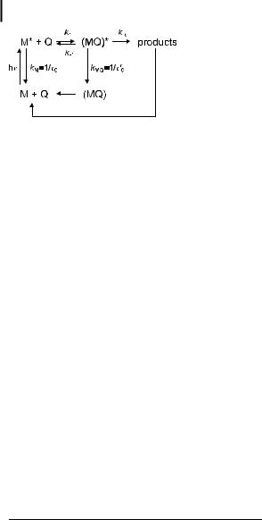
Case C is illustrated in Scheme 4.2, where k1 is the di usional second-order rate constant for the formation of the pair (M . . . Q) from separated M and Q,

k 1 is the first-order backward rate constant for this step, kR is the first-order rate constant for the reaction of (M . . . Q) to form ‘products’3), and kM ð¼ 1=t0Þ is the rate constant for intrinsic de-excitation of M . If the interaction between M and Q is weak, the fluorescence characteristics of the pair M . . . Q are the same as those of M (Scheme 4.2).

If the fluorescence of the pair is di erent from that of M (e.g. in the case of the formation of an exciplex (MQ) , which may be an intermediate in electron

transfer reactions; see Sections 4.3 and 4.4.2), a di erent rate constant kMQ ð¼ 1=t00 Þ for intrinsic de-excitation must be introduced (Scheme 4.3).

Scheme 4.2

3)For the sake of clarity, it is assumed that there is no back-reaction from the products to the pair.

76 4 Effects of intermolecular photophysical processes on fluorescence emission

Scheme 4.3

If Q is identical to M (self-quenching without formation of products), (MM) is called an excimer (excited dimer) with its own fluorescence spectrum and lifetime (Section 4.4.1).

A kinetic analysis of Schemes 4.2 and 4.3 shows that, in all cases, it is valid to consider a pseudo-first order rate constant kq½Q& and that three main cases should be considered:

1.kR gk1½Q&, k 1, 1=t0: the reaction is di usion-limited; the observed rate constant for quenching, kq, is equal to the di usional rate constant k1.

2.kR fk1½Q&, k 1 g1=t0: the equilibrium is reached prior to the formation of products.

3.kR is of the same order of magnitude or is smaller than the other rate constants: kq is smaller than k1 and can be written as

where p is the probability of reaction for the encounter pair (often called e - ciency), which can be expressed as a function of the rate constants (Eftink and Ghiron, 1981). For instance, p is close to 1 for oxygen, acrylamide and I , whereas it is less than 1 for succinimide, Br and IO3 . Examples of p and kq values are given in Tables 4.2 and 4.3.

Tab. 4.2. Examples of p and kq values for indole in the presence of various quenchers (from Eftink, 1991b)

4.2 Overview of the intermolecular de-excitation processes of excited molecules 77

Tab. 4.3. Examples of kq values for various fluorophore–quencher pairs (from Eftink, 1991b)

Abbreviations: PRODAN: 6-propionyl-2-(dimethylamino)naphthalene;

DENS: 6-diethylaminonaphthalene-1-sulfonic acid.

It should be emphasized that for di usion-controlled reactions, the observed rate constant for quenching is time-dependent. In fact, the excited fluorophores M that are at a short distance from a quencher Q at the time of excitation react, on average, at shorter times than those that are more distant, because mutual approach requires a longer time before reaction occurs. The important consequence of this is that the very beginning of fluorescence decay curves following pulse excitation will be a ected. Such transient e ects are not significant for moderate concentrations of quenchers in fluid solvents but they are noticeable at larger quencher concentrations and/or in viscous media. In steady-state experiments, it will be demonstrated that the consequence of these transient e ects is a departure from the well known and widely used Stern–Volmer plot. Stern–Volmer kinetics that ignore the transient e ects will be presented first.

4.2.2

Dynamic quenching

4.2.2.1 Stern–Volmer kinetics

As a first approach, the experimental quenching rate constant kq is assumed to be time-independent. According to the simplified Scheme 4.1, the time evolution of the concentration of M following a d-pulse excitation obeys the following di erential equation:

d½M & ¼ ðkM þ kq½Q&Þ½M & dt

¼ ð1=t0 þ kq½Q&Þ½M & ð4:3Þ

Integration of this di erential equation with the initial condition [M ] ¼ [M ]0 at t ¼ 0 yields:

78 4 Effects of intermolecular photophysical processes on fluorescence emission

The fluorescence intensity is proportional to the concentration of M and is given by

where kr is the radiative rate constant of M . The fluorescence decay is thus a single exponential whose time constant is

Time-resolved experiments in the absence and presence of quencher allow us to check whether the fluorescence decay is in fact a single exponential, and provide directly the value of kq. The fluorescence quantum yield in the presence of quencher is

Equations (4.8) and (4.9) lead to the Stern–Volmer relation:

where I0 and I are the steady-state fluorescence intensities (for a couple of wavelengths lE and lF) in the absence and in the presence of quencher, respectively. KSV ¼ kqt0 is the Stern–Volmer constant. Generally, the ratio I0=I is plotted against the quencher concentration (Stern–Volmer plot). If the variation is found to be linear, the slope gives the Stern–Volmer constant. Then, kq can be calculated if the excited-state lifetime in the absence of quencher is known.

80 4 Effects of intermolecular photophysical processes on fluorescence emission

Box 4.1 Theories of di usion-controlled reactions

The aim of this box is to present the most important expressions for the timedependent rate constant k1ðtÞ that have been obtained for a di usion-controlled reaction between A and B.

The d-pulse response of the fluorescence intensity can then be obtained by introducing the relation giving k1ðtÞ into Eq. (4.14) and by analytical or numerical integration of this equation.

Smoluchowski’s theorya)

Smoluchowski, who worked on the rate of coagulation of colloidal particles, was a pioneer in the development of the theory of di usion-controlled reactions. His theory is based on the assumption that the probability of reaction is equal to 1 when A and B are at the distance of closest approach ðRcÞ (‘absorbing boundary condition’), which corresponds to an infinite value of the intrinsic rate constant kR. The rate constant k 1 for the dissociation of the encounter pair can thus be ignored. As a result of this boundary condition, the concentration of B is equal to zero on the surface of a sphere of radius Rc, and consequently, there is a concentration gradient of B. The rate constant for reaction k1ðtÞ can be obtained from the flux of B, in the concentration gradient, through the surface of contact with A. This flux depends on the radial distribution function of B, pðr; tÞ, which is a solution of Fick’s equation

where r is the distance between A and B, and D is their mutual di usion coefficient (given by Eq. 4.12). The initial distribution of B is assumed to be uniform.

Under these conditions, the solution of Eq. (B4.1.1) is the Smoluchowski relation:

where N is Avogadro’s number divided by 1000.

Collins–Kimball’s theoryb)

In contrast to Smoluchowski’s theory, the rate constant for the intrinsic reaction has a finite value kR when A and B are at the distance of closest approach

4.2 Overview of the intermolecular de-excitation processes of excited molecules 81

ðr ¼ RcÞ, but it is equal to zero for larger distances. It is assumed that kR is proportional to the probability that a molecule B is located at a distance from A between Rc and Rc þ dr. Assuming that the rate constant k 1 for the dissociation of the encounter pair can still be ignored, the resolution of the di usion equation (B4.1.1) yields

Time-resolved fluorescence experiments carried out with 1,2-benzanthracene quenched by CBr4 in propane-1,2-diol show a better fit with the Collins–Kimball equation than with the Smoluchowski equation.

Cases of distance-dependent rate constants

1. Exponential distance dependence

In the Collins–Kimball theory, the rate constant for the reaction was assumed to be distance-independent. Further refinement proposed by Wilemski and Fixmanc) consists of considering that the reaction rate constant has an exponential dependence on distance, which is indeed predicted for electron transfer reactions and energy transfer via electron exchange (see Dexter’s formula in Section 4.6.3). The rate constant can thus be written in the following form:

The distance dependence is characterized by the parameter re, which is in the range 0.5–2 A˚ . The di usion equation (B4.1.2) must be modified by adding a distance-dependent sink term kðrÞ

For instance, very satisfactory fits of the experimental decay curves of coumarine 1 in the presence of aniline or N,N-dimethylaniline as quenchers were observed by Shannon and Eadsd) (with re ¼ 0:5 A˚ and Rc ¼ 5:5 A˚ ).

It should be noted that, in media of low viscosity, the transient term is significant only at short times (< 100 ps at viscosities similar to that of water) and can be neglected, whereas in viscous media, this term cannot be ignored (the fluorescence decay is then no longer a single exponential).

Under continuous illumination, the steady-state intensity can be easily calculated by considering a light of constant intensity as an infinite sum of infinitely short light pulses. It is thus simply obtained by integration of the d-pulse response. The ratio of the intensities in the absence and in the presence of quencher is then given by

with a and b given by Eqs (4.16) and (4.17), respectively. erfc is the complementary error function:

Equation (4.18) can be compared to the Stern–Volmer relation (4.10). The multiplying factor Y 1 accounts for the transient term and leads to a slight upward curvature of the Stern–Volmer plot.

At long times, the second term in Eq. (4.13) is negligible so that the decay becomes exponential with a decay time t given by

This relation is identical to Eq. (4.7) with kq ¼ 4pNRcD.

84 4 Effects of intermolecular photophysical processes on fluorescence emission

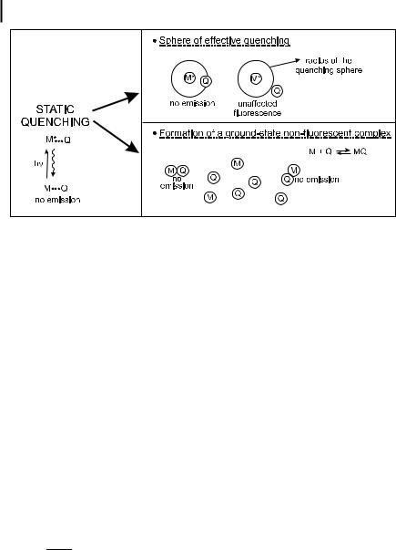
Fig. 4.1. Illustration of static quenching.

4.2.3

Static quenching

The term static quenching implies either the existence of a sphere of e ective quenching or the formation of a ground-state non-fluorescent complex (Figure 4.1) (Case A of Section 4.2.1).

4.2.3.1 Sphere of e ective quenching

When M and Q cannot change their positions in space relative to one another during the excited-state lifetime of M (i.e. in viscous media or rigid matrices), Perrin proposed a model in which quenching of a fluorophore is assumed to be complete if a quencher molecule Q is located inside a sphere (called the sphere of e ective quenching, active sphere or quenching sphere) of volume Vq surrounding the fluorophore M. If a quencher is outside the active sphere, it has no e ect at all on M. Therefore, the fluorescence intensity of the solution is decreased by addition of Q, but the fluorescence decay after pulse excitation is una ected.

The probability that n quenchers reside within this volume is assumed to obey a Poisson distribution:

where hni is the mean number of quenchers in the volume Vq: hni ¼ VqNa½Q& (Vq is expressed in L, ½Q& in mol L 1, Na is Avogadro’s number). The probability that there is no quencher in this volume is

Therefore, because the emission intensity is proportional to P0, Perrin’s model