Molecular Fluorescence

2.2 Probability of transitions. The Beer–Lambert Law. Oscillator strength 25

Box 2.1 Derivation of the Beer–Lambert Law and comments on its practical use

Derivation of the Beer–Lambert Law from considerations at a molecular scale is more interesting than the classical derivation (stating that the fraction of light absorbed by a thin layer of the solution is proportional to the number of absorbing molecules). Each molecule has an associated photon-capture area, called the molecular absorption cross-section s, that depends on the wavelength. A thin layer of thickness dl contains dN molecules. dN is given by

dN ¼ NacS dl

where S is the cross-section of the incident beam, c is the concentration of the solution and Na is Avogadro’s number. The total absorption cross-section of the thin layer is the sum of all molecular cross-sections, i.e. s dN. The probability of photon capture is thus s dN=S and is simply equal to the fraction of light ð dI=IÞ absorbed by the thin layer:

Integration leads to

where l is the thickness of the solution. This equation is formally identical to Eq. (2.2) with e ¼ Nas=2:303.

The molecular absorption cross-section can then be calculated from the experimental value of e using the following relation:

s ¼ 2:303e ¼ 3:825 10 19e ðin cm2Þ

Na

Practical use of the Beer–Lambert law deserves attention. In general, the sample is a cuvette containing a solution. The absorbance must be characteristic of the absorbing species only. Therefore, it is important to note that in the Beer–Lam- bert Law ðAðlÞ ¼ log I0=I ¼ eðlÞlcÞ, I0 is the intensity of the beam entering the solution but not that of the incident beam Ii on the cuvette, and I is the intensity of the beam leaving the solution but not that of the beam IS leaving the cuvette (see Figure B2.1). In fact, there are some reflections on the cuvette walls and these walls may also absorb light slightly. Moreover, the solvent is assumed to have no contribution, but it may also be partially responsible for a decrease in intensity because of scattering and possible absorption. The contributions of the

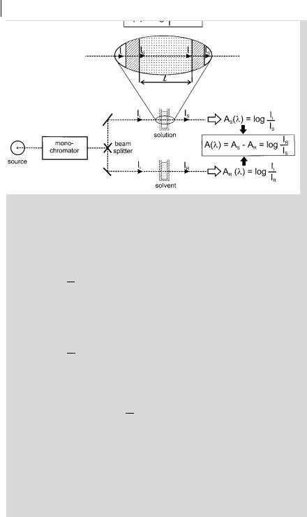
26 2 Absorption of UV–visible light

Fig. B2.1. Practical aspects of absorbance measurements.

cuvette walls and the solvent can be taken into account in the following way. The absorbance of the whole sample (including the cuvette walls) is defined as

ASðlÞ ¼ log Ii

IS

If the solution is replaced by the solvent, the intensity of the transmitted light is IR and the absorbance becomes

ARðlÞ ¼ log Ii

IR

The true absorbance of the solution is then given by

AðlÞ ¼ ASðlÞ ARðlÞ ¼ log IR

IS

As shown in Figure B2.1, double-beam spectrophotometers automatically record the true absorbance by measuring logðIR=ISÞ, thanks to a double compartment containing two cuvettes, one filled with the solution and one filled with the solvent. Because the two cuvettes are never perfectly identical, the baseline of the instrument is first recorded (with both cuvettes filled with the solvent) and stored. Then, the solvent of the sample cuvette is replaced by the solution, and the true absorption spectrum is recorded.

2.2 Probability of transitions. The Beer–Lambert Law. Oscillator strength 27

Tab. 2.1. Examples of molar absorption coefficients, e (at the wavelength corresponding to the maximum of the absorption band of lower energy). Only approximate values are given, because the value of e slightly depends on the solvent

value is 1. For n ! p transitions, the values of e are in the order of a few hundreds or less and those of f are no greater than @10 3. For p ! p transitions, the values of e and f are in principle much higher (except for symmetry-forbidden transitions): f is close to 1 for some compounds, which corresponds to values of e that are of the order of 105. Table 2.1 gives some examples of values of e.

In the quantum mechanical approach, a transition moment is introduced for characterizing the transition between an initial state and a final state (see Box 2.2). The transition moment represents the transient dipole resulting from the displacement of charges during the transition; therefore, it is not strictly a dipole moment.

The concept of transition moment is of major importance for all experiments carried out with polarized light (in particular for fluorescence polarization experiments, see Chapter 5). In most cases, the transition moment can be drawn as a vector in the coordinate system defined by the location of the nuclei of the atoms4); therefore, the molecules whose absorption transition moments are parallel to the electric vector of a linearly polarized incident light are preferentially excited. The probability of excitation is proportional to the square of the scalar product of the transition moment and the electric vector. This probability is thus maximum when the two vectors are parallel and zero when they are perpendicular.

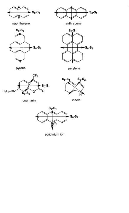
For p ! p transitions of aromatic hydrocarbons, the absorption transition moments are in the plane of the molecule. The direction with respect to the molecular axis depends on the electronic state attained on excitation. For example, in naphthalene and anthracene, the transition moment is oriented along the short axis for the S0 ! S1 transition and along the long axis for the S0 ! S2 transition. Various examples are shown in Figure 2.3.

4)Note that this is not true for molecules having a particular symmetry, such as benzene ðD6hÞ, triphenylene ðD3hÞ and C60

ðIhÞ.

28 2 Absorption of UV–visible light

Box 2.2 Einstein coe cients. Transition moment. Oscillator strength

Let us consider a molecule and two of its energy levels E1 and E2. The Einstein coe cients are defined as follows (Scheme B2.2): B12 is the induced absorption coe cient, B21 is the induced emission coe cient and A21 is the spontaneous emission coe cient.

Scheme B2.2

The coe cients for spontaneous and induced emissions will be discussed in Chapter 3 (see Box 3.2).

The rate at which energy is taken up from the incident light is given by

dPdt12 ¼ B12rðnÞ

where rðnÞ is the energy density incident on the sample at frequency n. B12 appears as the transition rate per unit energy density of the radiation. In the quantum mechanical theory, it is shown that

Ð

In this expression, hC1jMjC2i ¼ C1MC2 dt, where C1 and C2 are the wavefunctions of states 1 and 2, respectively, dt is over the whole configuration space of the 3N coordinates, M is the dipole moment operator (M ¼ Serj, where rj is the vector joining the electron j to the origin of a coordinate system linked to the molecule).

It should be noted that the dipole moment of the molecule in its ground state is hC1jMjC1i. In contrast, the term hC1jMjC2i is not strictly a dipole moment because there is a displacement of charges during the transition; it is called transition moment M12 that characterizes the transition.

It is interesting that there is a relation between the oscillator strength f (given by Eq. 2.6) and the square of the transition moment integral, which bridges the gap between the classical and quantum mechanical approaches:

f ¼ 8p2mn jhC1jMjC2ij2

3he2

Note also that the oscillator strength can be related to the coe cient B12:

mhn

f ¼ pe2 B12

For more details, see Birks (1970), pp. 48–52.

302 Absorption of UV–visible light

2.3

Selection rules

There are two major selection rules for absorption transitions:

1.Spin-forbidden transitions. Transitions between states of di erent multiplicities are forbidden, i.e. singlet–singlet and triplet–triplet transitions are allowed, but singlet–triplet and triplet–singlet transitions are forbidden. However, there is always a weak interaction between the wavefunctions of di erent multiplicities

via spin–orbit coupling5). As a result, a wavefunction for a singlet (or triplet) state always contains a small fraction of a triplet (or singlet) wavefunction C ¼ a1C þ b3C; this leads to a small but non-negligible value of the intensity integral during a transition between a singlet state and a triplet state or vice versa (see Scheme 2.1). In spite of their very small molar absorption coe cients, such transitions can be e ectively observed.

Intersystem crossing (i.e. crossing from the first singlet excited state S1 to the first triplet state T1) is possible thanks to spin–orbit coupling. The e ciency of this coupling varies with the fourth power of the atomic number, which explains why intersystem crossing is favored by the presence of a heavy atom. Fluorescence quenching by internal heavy atom e ect (see Chapter 3) or external heavy atom e ect (see Chapter 4) can be explained in this way.

2.Symmetry-forbidden transitions. A transition can be forbidden for symmetry reasons. Detailed considerations of symmetry using group theory, and its consequences on transition probabilities, are beyond the scope of this book. It is important to note that a symmetry-forbidden transition can nevertheless be observed because the molecular vibrations cause some departure from perfect symmetry (vibronic coupling). The molar absorption coe cients of these transitions are very small and the corresponding absorption bands exhibit welldefined vibronic bands. This is the case with most n ! p transitions in solvents that cannot form hydrogen bonds (e A100–1000 L mol 1 cm 1).

2.4

The Franck–Condon principle

According to the Born–Oppenheimer approximation, the motions of electrons are much more rapid than those of the nuclei (i.e. the molecular vibrations). Promotion of an electron to an antibonding molecular orbital upon excitation takes about 10 15 s, which is very quick compared to the characteristic time for molecular vi-

2.4 The Franck–Condon principle 31

Box 2.3 Classical and quantum mechanical description of the Franck–Condon principlea)

Classically, the transition occurs when the distances between nuclei are equal to the equilibrium bond lengths of the molecule in the ground state. While the transition is in progress, the position of the nuclei is unchanged and they do not accelerate. Consequently, the transition terminates where the vertical line intersects the potential energy curve of the lowest excited state, i.e. at the turning point. As soon as the transition is complete, the excited molecule begins to vibrate at an energy corresponding to the intersection.

In the quantum mechanical description (in continuation of Box 2.2), the wavefunction can be described by the product of an electronic wavefunction C and a vibrational wavefunction w (the rotational contribution can be neglected), so that the probability of transition between an initial state defined by C1wa and a final state defined by C2wb is proportional to jhC1wajMjC2wbij2. Because M only depends on the electron coordinates, this expression can be rewritten as the product of two terms jhC1jMjC2ij2jhwa j wbij2 where the second term is called the Franck–Condon factor. Qualitatively, the transition occurs from the lowest vibrational state of the ground state to the vibrational state of the excited state that it most resembles in terms of vibrational wavefunction.

a)Atkins P. W. and Friedman R. S. (1997)

Molecular Quantum Mechanics, Oxford University Press, Oxford.

brations (10 10 –10 12 s). This observation is the basis of the Franck–Condon principle: an electronic transition is most likely to occur without changes in the positions of the nuclei in the molecular entity and its environment (Box 2.3). The resulting state is called a Franck–Condon state, and the transition is called vertical transition, as illustrated by the energy diagram of Figure 2.4 in which the potential energy curve as a function of the nuclear configuration (internuclear distance in the case of a diatomic molecule) is represented by a Morse function.

At room temperature, most of the molecules are in the lowest vibrational level of the ground state (according to the Boltzmann distribution; see Chapter 3, Box 3.1). In addition to the ‘pure’ electronic transition called the 0–0 transition, there are several vibronic transitions whose intensities depend on the relative position and shape of the potential energy curves (Figure 2.4).

The width of a band in the absorption spectrum of a chromophore located in a particular microenvironment is a result of two e ects: homogeneous and inhomogeneous broadening. Homogeneous broadening is due to the existence of a continuous set of vibrational sublevels in each electronic state. Inhomogeneous broadening results from the fluctuations of the structure of the solvation shell

32 2 Absorption of UV–visible light

Fig. 2.4. Top: Potential energy diagrams with vertical transitions (Franck–Condon principle). Bottom: shape of the absorption bands; the vertical broken lines represent the absorption lines that are observed for a vapor, whereas broadening of the spectra is expected in solution (solid line).

surrounding the chromophore. Such broadening e ects exist also for emission bands in fluorescence spectra and will be discussed in Section 3.5.1.

Shifts in absorption spectra due to the e ect of substitution or a change in environment (e.g. solvent) will be discussed in Chapter 3, together with the e ects on emission spectra. Note that a shift to longer wavelengths is called a bathochromic shift (informally referred to as a red-shift). A shift to shorter wavelengths is called a hypsochromic shift (informally referred to as a blue-shift). An increase in the molar absorption coe cient is called the hyperchromic e ect, whereas the opposite is the hypochromic e ect.