

Molecular Fluorescence
.pdf5.5 Case of motionless molecules with random orientation 135
where K is a proportionality factor. The bars characterize an ensemble average over the N emitting molecules at time t.
Because of the axial symmetry around Oz, a2ðtÞ ¼ b2ðtÞ, and because a2ðtÞ þ
|
|
|
|
|
|
|
|
|
|
|
|
|
|
|
|
|
|
|
|
|
b2ðtÞ þ |
g2ðtÞ ¼ 1, |
we have g2ðtÞ ¼ 1 2a2ðtÞ. The emission |
anisotropy is |
then |
||||||||||||||||
given by |
|
|
|
|
|
|
|
|
|
|
|
|
|
|
|
|
|
|||
|
rðtÞ ¼ |
IkðtÞ I? |
ðtÞ |
|
IzðtÞ IyðtÞ |
|
|
|||||||||||||
|
|
|
|
|
|
|
¼ |
|
|
|
|
|
|
|
||||||
|
|
|
|
IðtÞ |
|
IxðtÞ þ IyðtÞ þ IzðtÞ |
|
|
||||||||||||
|
|
|
|
|
|
|
|
|
|
|
|
|
|
|
||||||
|
|
|
|
|
|
|
|
|
|
|
3g2ðtÞ 1 |
|
|
|
||||||
¼ |
g2 |
t |
a2 |
t |
ð |
5:19 |
||||||||||||||
|
ð Þ |
|
ð Þ ¼ |
2 |
|
|
|
|
Þ |
|||||||||||
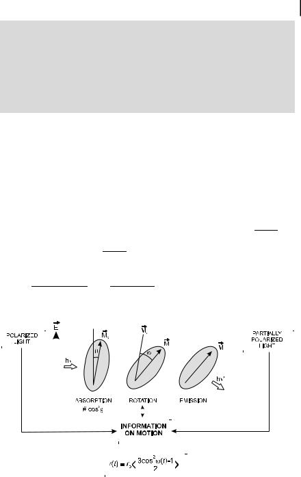
Finally, because g ¼ cos yE, the relation between the emission anisotropy and the angular distribution of the emission transition moments can be written as
|
|
|
|
|
|
r t |
3 cos2 yEðtÞ 1 |
ð |
5:20 |
||
ð Þ ¼ |
2 |
|
Þ |
||
5.5
Case of motionless molecules with random orientation
5.5.1
Parallel absorption and emission transition moments
When the absorption and emission transition moments are parallel, yA ¼ yE, the
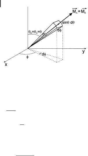
common value being denoted y; hence cos2 yA ¼ cos2 yE ¼ cos2 y. Before excitation, the number of molecules whose transition moment is oriented within angles y and y þ dy, and f and f þ df is proportional to an elementary surface on a sphere whose radius is unity, i.e. 2p sin y dy df (Figure 5.6).
Taking into account the excitation probability, i.e. cos2 y, the number of excited molecules whose transition moment is oriented within angles y and y þ dy, and f and f þ df, is proportional to cos2 y sin y dy df. The fraction of molecules oriented in this direction is
cos2 y sin y dy df |
|
Wðy; fÞ dy df ¼ Ð02p df Ð0p cos2 y sin y dy |
ð5:21Þ |
The denominator, which is proportional to the total number of excited molecules, can be calculated by setting x ¼ cos y, hence dx ¼ sin y dy, and its value is 4p=3. Equation (5.21) then becomes
Wðy; fÞ dy df ¼ |
3 |
cos2 y sin y dy df |
ð5:22Þ |
4p |
136 5 Fluorescence polarization. Emission anisotropy
Fig. 5.6. The fraction of molecules whose absorption and emission transition moments are parallel and oriented in a direction within the elementary solid angle. This direction is defined by angles y and f.
It is then possible to calculate the average of cos2 y over all excited molecules
ð2p ðp
cos2 y ¼ df cos2 yWðy; fÞ dy
00
¼3 ð2p df ðp cos4 y sin y dy
4p 0 0
|
|
|
¼ 3=5 |
|
|
|
|
|
|
|
ð5:23Þ |
||
Using Eq. (5.20), the emission anisotropy can thus be written as |
|
|
|||||||||||
|
|
|
|
|
|
|
|
|
|
|
|
|
|
|
|
|
|
|
|
|
|
|
|
|
|
|
|
|
r |
¼ |
3 cos2 y 1 |
¼ |
2 |
¼ |
0:4 |
|
ð |
5:24 |
|||
|
|
|
|
||||||||||
|
2 |
|
5 |
|
|||||||||
|
0 |
|
|
|
Þ |
||||||||
r0 is called the fundamental anisotropy, i.e. the theoretical anisotropy in the absence of any motion. In practice, rotational motions can be hindered in a rigid medium. The experimental value, called the limiting anisotropy, turns out to be always slightly smaller than the theoretical value. When the absorption and emission transition moments are parallel, i.e. when the molecules are excited to the first singlet state, the theoretical value of r0 is 0.46), but the experimental value usually ranges from 0.32 to 0.39. The reasons for these di erences are discussed in Box 5.1.
6)The corresponding value of the polarization ratio is p0 ¼ 0:5.

5.5 Case of motionless molecules with random orientation 137
Box 5.1 Fundamental and limiting anisotropies
The di erence between the theoretical value of the emission anisotropy in the absence of motions ( fundamental anisotropy) and the experimental value (limiting anisotropy) deserves particular attention. The limiting anisotropy can be determined either by steady-state measurements in a rigid medium (in order to avoid the e ects of Brownian motion), or time-resolved measurements by taking the value of the emission anisotropy at time zero, because the instantaneous anisotropy can be written in the following form:
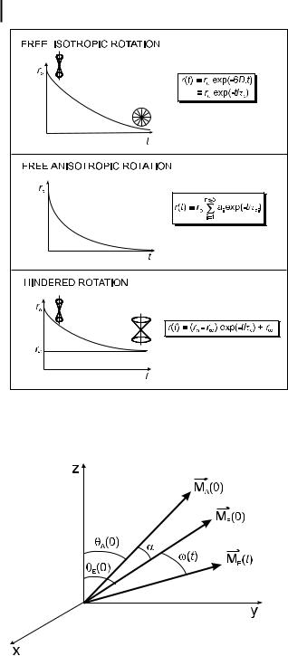
rðtÞ ¼ r0 f ðtÞ
where f ðtÞ characterizes the dynamics of rotational motions (orientation autocorrelation function) (see Section 5.6, Eq. 5.32) and whose value is 1 at time zero.
It should first be noted that the measurement of emission anisotropy is di - cult, and instrumental artefacts such as large cone angles of the incident and/or observation beams, imperfect or misaligned polarizers, re-absorption of fluorescence, optical rotation, birefringence, etc., might be partly responsible for the di erence between the fundamental and limiting anisotropies.
If there is no significant instrumental artefact, any observed di erence must be related to the fluorophore itself. There may be several causes. Firstly, a trivial e ect can be the overlap of low-lying absorption bands, resulting in an anomalous excitation polarization spectrum. Secondly, the oscillator associated with absorption may not be strictly linear, but may be partly two-dimensional or three-dimensional. However, it is generally considered that the di erence between the fundamental and limiting anisotropies is mainly due to torsional vibrations of the fluorophores about their equilibrium orientation, as first suggested by Jablonskia). A temperature dependence of the limiting anisotropy is then expected, and was indeed reportedb,c): at low temperature (i.e. when the medium is frozen), r0 may be considered as a constant quantity whereas at high temperature it decreases linearly with the temperature.
Fast librational motions of the fluorophore within the solvation shell should also be consideredd). The estimated characteristic time for perylene in para n is about 1 ps, which is not detectable by time-resolved anisotropy decay measurement. An ‘apparent’ value of the emission anisotropy is thus measured, which is smaller than in the absence of libration. Such an explanation is consistent with the fact that fluorescein bound to a large molecule (e.g. polyacrylamide or monoglucoronide) exhibits a larger limiting anisotropy than free fluorescein in aqueous glycerolic solutions. However, the absorption and fluorescence spectra are di erent for free and bound fluorescein; the question then arises as to whether r0 could be an intrinsic property of the fluorophore.
In this respect, Johanssone) reported that r0 is the same (within experimental accuracy) for fluorophores belonging to the same family, e.g. perylene and perylenyl compounds ð0:369 G0:002Þ, or xanthene derivatives such as rhodamine

138 5 Fluorescence polarization. Emission anisotropy
B, rhodamine 6G, rhodamine 101 and fluorescein ð0:373 G0:002Þ. Therefore, r0 appears to be an intrinsic property of a fluorophore related to its structure and to the shape of its absorption and fluorescence spectra. A possible explanation for a limiting anisotropy being less than the fundamental anisotropy could then be a change of the molecular geometry between the ground and excited states. In fact, the aromatic plane of perylene was suggested to be slightly twisted in the ground state, and evidence of butterfly-type intramolecular folding in xanthene dyes has been reported.
a)Jablonski A. (1950) Acta Phys. Pol. 10, 193.
b)Kawski A., Kubicki A. and Weyna I. (1985)
Z. Naturforsch. 40a, 559.
c)Veissier V., Viovy J. L. and Monnerie L.
(1989) J. Phys. Chem. 93, 1709.
d)Zinsli P. E. (1977) Chem. Phys. 93, 1989.
e)Johansson L. B. (1990) J. Chem. Soc. Faraday Trans. 86, 2103.
5.5.2
Non-parallel absorption and emission transition moments
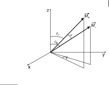
This situation occurs when excitation brings the fluorophores to an excited state other than the first singlet state from which fluorescence is emitted. Let a be the angle between the absorption and emission transition moments. The aim is to calculate cos yE and then to deduce r by means of Eq. (5.20).
According to the classical formula of spherical trigonometry, cos yE can be written as
cos yE ¼ cos yA cos a þ cos c sin yA sin a |
ð5:25Þ |
where c denotes the angle between the planes ðOz; MAÞ and ðOz; MEÞ (Figure 5.7). By taking the square of the two sides of Eq. (5.25) and taking into account the
fact that all values of c are equiprobable ðcos c ¼ 0; cos2 c ¼ 1=2Þ, we obtain
|
|
|
|
|
|
|
|
|
|
|
|
|
|
|
1 |
|
|
|
|
|
|
|
|
|
|
|
|
|
|
|
|
|
|
|
|
|
|
|
|
|
|
|
|
|
|
|
|
|
|
|
|
|
|
|
|
|
|
|
|
|
|
|
|
|
|
|
|
|
|
|
|
||
|
cos2 yE ¼ cos2 a cos2 |
yA þ |
|
sin2 a sin2 yA |
|
|
|
|
|
|
|
|||||||||||||||||||||||||
|
|
|
|
|
|
|
|
|
|
|
||||||||||||||||||||||||||
|
2 |
|
|
|
|
|
|
|
|
|||||||||||||||||||||||||||
|
|
|
|
|
|
|
|
|
|
|
|
|
|
|
1 |
|
|
|
|
|
|
|
|
|
|
|
|
|
|
|
|
|
|
|
|
|
|
|
|
|
|
¼ cos2 a cos2 |
yA þ |
ð1 cos2 aÞð1 cos2 yAÞ |
|
|
|||||||||||||||||||||||||||
|
|
|
|
|
|
|
|
|
||||||||||||||||||||||||||||
|
|
|
|
|
2 |
|
|
|||||||||||||||||||||||||||||
|
|
|
3 |
|
|
|
|
|
|
|
|
|
|
|
1 |
|
|
|
|
1 |
|
|
|
|
|
|
1 |
|
|
|||||||
|
|
|
cos2 a cos2 yA |
|
|
|
|
|
cos2 a þ |
|
|
|||||||||||||||||||||||||
|
|
|
|
|
¼ |
|
|
|
|
cos2 yA |
|
|
|
ð5:26Þ |
||||||||||||||||||||||
|
|
|
|
|
2 |
2 |
2 |
2 |
||||||||||||||||||||||||||||
Hence |
|
|
|
|
|
|
|
|
|
|
|
|
|
|
|
|
|
|
|
|
|
|
|
|
|
|
|
|
|
|
|
|
|
|
||
|
|
|
|
|
|
|
|
|
|
|
|
|
|
|
|
|
|
|
||||||||||||||||||
|
r |
|
3 cos2 yE |
1 |
|
3 cos2 yA |
1 |
|
3 cos2 a 1 |
|
|
|
5:27 |
|||||||||||||||||||||||
|
0 ¼ |
2 |
¼ |
|
|
|
|
2 |
|
|
|
|
|
|
|
|
|
ð |
||||||||||||||||||
|
|
|
|
|
|
|
|
|
|
2 |
|
|
|
|
|
Þ |
||||||||||||||||||||
Because cos2 yA ¼ 3=5, the emission anisotropy is given by
5.5 Case of motionless molecules with random orientation 139
Fig. 5.7. Definition of angles a and c when the absorption and emission transition moments are not parallel.
|
|
|
|
|
|
|
|
|
|
|
|
|
|
|
|
|
|
|
|
|
|
|
|
|
|
|
|
|
|
r |
¼ |
2 |
3 cos2 a 1 |
|
5:28 |
||||
5 |
2 |
|
|||||||
0 |
|
|
ð Þ |
||||||
Consequently, the theoretical values of r0 range from 2=5 ð¼ 0:4Þ for a ¼ 0 (parallel transition moments) and 1=5 ð¼ 0:2Þ for a ¼ 90 (perpendicular transition moments)7):
0:2 ar0 a0:4 |
ð5:29Þ |
A value close to 0:2 is indeed observed in the case of some aromatic molecules excited to the second singlet state whose transition moment is perpendicular to that of the first singlet state from which fluorescence is emitted (e.g. perylene). r0 varies with the excitation wavelength for a given observation wavelength and these variations represent the excitation polarization spectrum, which allows us to distinguish between electronic transitions. Negative values generally correspond to S0 ! S2 transitions. As an illustration, Figure 5.8 shows the excitation polarization spectrum of perylene.
The case of indole and tryptophan is peculiar because the low-lying absorption bands overlap. Box 5.2 shows how the indole absorption spectrum can be resolved into two bands from the combined measurement of the excitation spectrum and the excitation polarization spectrum.
Particular cases should also be mentioned:
.For planar aromatic molecules with a symmetry axis of order 3 or higher (e.g. triphenylene: D ), r cannot exceed 0.1.
.The fluorescence emitted by fullerene ðC60Þ is intrinsically totally depolarized because of its almost perfect spherical symmetry ðIhÞ.
7)For the polarization ratio: 1=3 ap0 a1=23h 0
140 5 Fluorescence polarization. Emission anisotropy
Fig. 5.8. Excitation polarization spectrum of perylene in propane-1,2-diol at 60 C.
5.6
E ect of rotational Brownian motion
If excited molecules can rotate during the excited-state lifetime, the emitted fluorescence is partially (or totally) depolarized (Figure 5.9). The preferred orientation of emitting molecules resulting from photoselection at time zero is indeed gradually a ected as a function of time by the rotational Brownian motions. From the extent of fluorescence depolarization, we can obtain information on the molecular motions, which depend on the size and the shape of molecules, and on the fluidity of their microenvironment.
Quantitative information can be obtained only if the time-scale of rotational motions is of the order of the excited-state lifetime t. In fact, if the motions are slow with respect to tðr Ar0Þ or rapid ðr A0Þ, no information on motions can be obtained from emission anisotropy measurements because these motions occur out of the experimental time window.
A distinction should be made between free rotation and hindered rotation. In the case of free rotation, after a d-pulse excitation the emission anisotropy decays from r0 to 0 because the rotational motions of the molecules lead to a random orientation at long times. In the case of hindered rotations, the molecules cannot become randomly oriented at long times, and the emission anisotropy does not decay to zero but to a steady value, r (Figure 5.10). These two cases of free and hindered rotations will now be discussed.
5.6 Effect of rotational Brownian motion 141
Box 5.2 Resolution of the absorption spectrum of indolea)
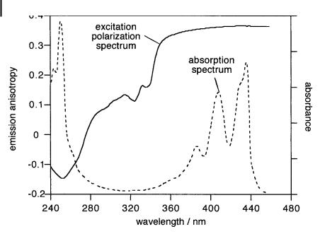
The long wavelength absorption band of indole consists of two electronic transitions 1La and 1Lb, whose transition moments are almost perpendicular (more precisely, they are oriented at 38 and 56 to the long molecular axis, respectively). Figure B5.2.1 shows the excitation spectrum and the excitation polarization spectrum in propylene glycol at 58 C.
The emission anisotropy r0ðlÞ at a wavelength of excitation l results from the addition of contributions from the 1La and 1Lb excited states with fractional contributions faðlÞ and f bðlÞ, respectively. According to the additivity law of emission anisotropies, r0ðlÞ is given by
r0ðlÞ ¼ faðlÞr0a þ f bðlÞr0b
with
faðlÞ þ f bðlÞ ¼ 1
Fig. B5.2.1. Corrected excitation spectrum (broken line) and excitation polarization spectrum of indole in propylene glycol at 58 C. The fluorescence is observed through a cut-o filter (Corning 7–39 filter) (reproduced with permission from Valeur and Webera)).

142 5 Fluorescence polarization. Emission anisotropy
where r0a and r0b are the limiting anisotropies corresponding to the 1La and 1Lb states when excited independently. In the long-wavelength region of the spectrum (305–310 nm), the 1La level is exclusively excited and the limiting anisotropy for this state is thus r0a ¼ 0:3 (instead of 0.4, for the reasons given in Box 5.1). Then, using Eq. (5.28), in which 0.4 ð2=5Þ is replaced by 0.3 and a is equal to 90 , we obtain
r0b ¼ 0:3 3 cos2 a 1 ¼ 0:15 2
The fractional contributions of the 1La and 1Lb excited states to the emission anisotropies are given by
f |
|
|
l |
r0ðlÞ r0b |
¼ |
r0ðlÞ þ 0:15 |
|
|
|
|
r0a r0b |
|
|||
|
a |
ð Þ ¼ |
|
0:45 |
|||
f |
|
|
l |
|
r0a r0ðlÞ |
0:3 r0ðlÞ |
|
|
b |
ð Þ ¼ |
|
r0a r0b |
¼ |
0:45 |
|
Finally, the contributions IaðlÞ and IbðlÞ of the 1La and 1Lb bands to the excitation spectrum IðlÞ are
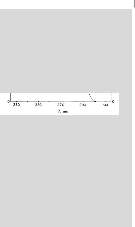
Fig. B5.2.2. Resolution of the excitation spectrum of indole (reproduced with permission from Valeur and Webera)).
5.6 Effect of rotational Brownian motion 143
IaðlÞ ¼ faðlÞIðlÞ
IbðlÞ ¼ fbðlÞIðlÞ
Figure B5.2.2 shows the resolution of the excitation spectrum. The 1Lb band lies below the broader 1La band and exhibits a vibrational structure.
a)Valeur B. and Weber G. (1977) Photochem. Photobiol. 25, 441.
5.6.1
Free rotations
The Brownian rotation of the emission transition moment is characterized by the angle oðtÞ through which the molecule rotates between time zero (d-pulse excitation) and time t, as shown in Figure 5.11.
Using the same method that led to Eq. (5.27), it is easy to establish the rule of multiplication of depolarization factors: when several processes inducing succes-
sive rotations of the transition moments (each being characterized by cos2 ziÞ are independent random relative azimuths, the emission anisotropy is the product of the depolarization factors ð3 cos2 zi 1Þ=2:
|
|
|
|
|
|
|
|
|
|
|
|
|
|
|
|
|
|
|
|
|
|
|
|
3 cos |
2 |
y |
|
|
3 cos |
2 z |
|
|
|
|
|
|
|
|
|||||||
rðtÞ ¼ |
|
EðtÞ 1 |
¼ |
Yi |
|
|
i 1 |
|
|
|
|
|
ð5:30Þ |
|||||||||
|
|
|
|
|
|
|
|
|
||||||||||||||
|
|
|
|
2 |
|
|
|
|
2 |
|
|
|
||||||||||
|
|
|
|
|
|
|
|
|
|
|
|
|
|
|
|
|
|
|
|
|
|
|
|
|
|
|
|
|
|
|
|
|
|
|
|
|
|
|
|
|
|
|
|
|
|
|
|
|
|
|
|
|
|
|
|
|
|
|
|
|
|
|
|
|
|
|
|
|
|
|
|
|
|
|
|
|
|
|
|
|
|
|
|
|
|
|
|
|
|
|
|
|
|
|
|
|
|
|
|
|
|
|
|
|
|
|
|
|
|
|
|
|
|
|
|
|
|
|
|
|
|
|
|
|
|
|
|
|
|
|
|
|
|
|
|
|
|
|
|
|
|
|
|
|
|
|
|
|
|
|
|
|
|
|
|
|
|
|
|
|
|
|
|
|
|
|
|
|
|
|
|
|
|
|
|
|
|
|
|
|
|
|
|
|
|
|
|
|
|
|
|
|
|
|
|
|
|
|
|
|
|
|
|
|
|
|
|
|
|
|
|
|
|
|
|
|
|
|
|
|
|
|
|
|
|
|
|
|
|
|
|
|
|
|
|
|
|
|
|
|
|
|
|
|
|
|
|
|
|
|
|
|
|
|
|
|
|
|
|
|
|
|
|
|
|
|
|
|
|
|
|
|
|
|
|
|
|
|
|
|
|
|
|
|
|
|
|
|
|
|
|
|
|
|
|
|
|
|
|
|
|
|
|
|
|
|
|
|
|
|
|
|
|
|
|
|
|
|
|
|
|
Fig. 5.9. Rotational motions inducing depolarization of fluorescence. The absorption and emission transition moments are assumed to be parallel.
144 5 Fluorescence polarization. Emission anisotropy
Fig. 5.10. Decay of emission anisotropy in the case of free and hindered rotations.
Fig. 5.11. Brownian rotation characterized by oðtÞ.