

Molecular Fluorescence
.pdfMolecular Fluorescence: Principles and Applications. Bernard Valeur
> 2001 Wiley-VCH Verlag GmbH
ISBNs: 3-527-29919-X (Hardcover); 3-527-60024-8 (Electronic)
125
5
Fluorescence polarization. Emission anisotropy
Polarisation de la lumie`re: Disposition des parties composant un rayon lumineux de sorte qu’elles se comportent toutes de la meˆme fac¸on.
Encyclope´die Me´thodique. Physique Monge, Cassini, Bertholon et al., 1822
[Polarization of light: Arrangement of the parts which make up a light ray so that they all act in the same way.]
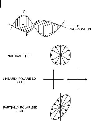
Light is an electromagnetic wave consisting of an electric field E and a magnetic field B perpendicular both to each other and to the direction of propagation, and oscillating in phase. For natural light, these fields have no preferential orientation, but for linearly polarized light, the electric field oscillates along a given direction; the intermediate case corresponds to partially polarized light (Figure 5.1).
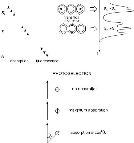
Most chromophores absorb light along a preferred direction1) (see Chapter 2 for the definition of absorption transition moment, and for examples of transition moments of some fluorophores, see Figure 2.3), depending on the electronic state. In contrast, the emission transition moment is the same whatever the excited state reached by the molecule upon excitation, because of internal conversion towards the first singlet state (Figure 5.2).
If the incident light is linearly polarized, the probability of excitation of a chromophore is proportional to the square of the scalar product MA.E, i.e. cos2 yA, yA being the angle between the electric vector E of the incident light and the absorption transition moment MA (Figure 5.2). This probability is maximum when E is parallel to MA of the molecule; it is zero when the electric vector is perpendicular.
1)The absorption transition moment is not in a single direction for some molecules whose
symmetry is D6h (benzene), D3h (triphenylene) or IhðC60Þ.
126 5 Fluorescence polarization. Emission anisotropy
Fig. 5.1. Natural light and linearly polarized light.
Thus, when a population of fluorophores is illuminated by a linearly polarized incident light, those whose transition moments are oriented in a direction close to that of the electric vector of the incident beam are preferentially excited. This is called photoselection. Because the distribution of excited fluorophores is anisotropic, the emitted fluorescence is also anisotropic. Any change in direction of the transition moment during the lifetime of the excited state will cause this anisotropy to decrease, i.e. will induce a partial (or total) depolarization of fluorescence.
The causes of fluorescence depolarization are:
. non-parallel absorption and emission transition moments
. torsional vibrations
. Brownian motion
. transfer of the excitation energy to another molecule with di erent orientation.
Fluorescence polarization measurements can thus provide useful information on molecular mobility, size, shape and flexibility of molecules, fluidity of a medium, and order parameters (e.g. in a lipid bilayer)2).
2)Circular polarized luminescence (CPL) is not covered in this book because the field of application of this phenomenon is limited to chiral systems that emit di erent amounts of left and right circularly polarized light. Nevertheless, it is worth mentioning that
valuable information can be obtained by CPL spectroscopy on the electronic and molecular structure in the excited state of chiral organic molecules, inorganic complexes and biomacromolecules (for a review, see Riehl J. P. and Richardson F. S. (1986) Chem. Rev. 86, 1).
5.1 Characterization of the polarization state of fluorescence (polarization ratio, emission anisotropy) |
127 |
||||||||||||||
|
|
|
|
|
|
|
|
|
|
|
|
|
|
|
|
|
|
|
|
|
|
|
|
|
|
|
|
|
|
|
|
|
|
|
|
|
|
|
|
|
|
|
|
|
|
|
|
|
|
|
|
|
|
|
|
|
|
|
|
|
|
|
|
|
|
|
|
|
|
|
|
|
|
|
|
|
|
|
|
|
|
|
|
|
|
|
|
|
|
|
|
|
|
|
|
|
|
|
|
|
|
|
|
|
|
|
|
|
|
|
|
|
|
|
|
|
|
|
|
|
|
|
|
|
|
|
|
|
|
|
|
|
|
|
|
|
|
|
|
|
|
|
|
|
|
|
|
|
|
|
|
|
|
|
|
|
|
|
|
|
|
|
|
|
|
|
|
|
|
|
|
|
|
|
|
|
|
|
|
|
|
|
|
|
|
|
|
|
|
|
|
|
|
|
|
|
|
|
|
|
|
|
|
|
|
|
|
|
|
|
|
|
|
|
|
|
|
|
|
|
|
|
|
|
|
|
|
|
|
|
|
|
|
|
|
|
|
|
|
|
|
|
|
|
|
|
|
|
|
|
|
|
|
|
|
|
|
|
|
|
|
|
|
|
|
|
|
|
|
|
|
|
|
|
|
|
|
|
|
|
|
|
|
|
|
|
|
|
|
|
|
|
|
|
|
|
|
|
|
|
|
|
|
Fig. 5.2. Transition moments (e.g. anthracene) and photoselection.
5.1
Characterization of the polarization state of fluorescence (polarization ratio, emission anisotropy)
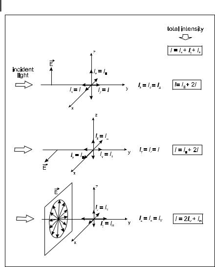
Because there is no phase relation between the light emitted by di erent molecules, fluorescence can be considered as the result of three independent sources of light polarized along three perpendicular axis Ox, Oy, Oz without any phase relation between them. Ix, Iy, Iz are the intensities of these sources, and the total intensity is I ¼ Ix þ Iy þ Iz. The values of the intensity components depend on the polarization of the incident light and on the depolarization processes. Application of the Curie symmetry principle (an e ect cannot be more dissymmetric than the
128 5 Fluorescence polarization. Emission anisotropy
Fig. 5.3. Relations between the fluorescence intensity components resulting from the Curie symmetry principle. The fluorescent sample is placed at the origin of the system of coordinates.
cause from which it results) leads to relations between intensity components, as shown in Figure 5.3. It should be noted that the symmetry principle is strictly valid only for a point source of light, which cannot be rigorously achieved in practice. Moreover, only homogeneous diluted solutions will be considered in this chapter, so that artefacts due for instance to inner filter e ects are avoided.
The various cases of excitation are now examined (Figure 5.3).
5.1 Characterization of the polarization state of fluorescence (polarization ratio, emission anisotropy) 129
5.1.1
Excitation by polarized light
5.1.1.1 Vertically polarized excitation
When the incident light is vertically polarized, the vertical axis Oz is an axis of symmetry for the emission of fluorescence according to the Curie principle, i.e. Ix ¼ Iy. The fluorescence observed in the direction of this axis is thus unpolarized.
The components of the fluorescence intensity that are parallel and perpendicular to the electric vector of the incident beam are usually denoted as Ik and I?, respectively. For vertically polarized incident light, Iz ¼ Ik and Ix ¼ Iy ¼ I?.
The intensity component Iz corresponding to oscillations of the electric field along the Oz axis cannot be detected by the eye or by a detector placed along this axis. The fluorescence intensity observed in the direction of this axis is thus
Ix þ Iy ¼ 2I?.
On the contrary, the Ox and Oy axes are not axes of symmetry for the emission of fluorescence. When fluorescence is observed through a polarizer along the Ox axis (or the Oy axis), the intensity measured is Iz ¼ Ik for the vertical position of the polarizer, and Iy ¼ I? (or Ix ¼ I?) for the horizontal position. Without polarizer, the measured intensity is Iz þ Iy ¼ Ik þ I? in the Ox direction and Iz þ Ix ¼ Ik þ I? in the Oy direction.
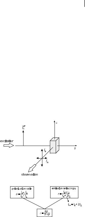
In most cases, fluorescence is observed in a horizontal plane at 90 to the propagation direction of the incident beam, i.e. in direction Ox (Figure 5.4). The fluorescence intensity components Ik and I? are measured by a photomultiplier in
Fig. 5.4. Usual configuration for measuring fluorescence polarization.

130 |
5 Fluorescence polarization. Emission anisotropy |
|
|||||
|
front of which a |
polarizer is rotated. The total fluorescence intensity is I |
¼ |
||||
|
|||||||
|
3) |
. |
|||||
|
Ix þ Iy þ Iz ¼ Ik þ 2I? |
|
|||||
|
The polarization state of fluorescence is characterized either by |
|
|||||
|
. the polarization ratio p: |
|
|||||
|
|
p ¼ |
Ik I? |
|
ð5:1Þ |
||
|
|
Ik þ I? |
|
|
|||
. or the emission anisotropy r:
Ik I? |
|
r ¼ Ik þ 2I? |
ð5:2Þ |
In the expression of the polarization ratio, the denominator represents the fluorescence intensity in the direction of observation, whereas in the formula giving the emission anisotropy, the denominator represents the total fluorescence intensity. In a few situations (e.g. the study of radiative transfer) the polarization ratio is to be preferred, but in most cases, the use of emission anisotropy leads to simpler relations (see below).
The relationship between r and p follows from Eqs (5.1) and (5.2):
r ¼ |
2p |
ð5:3Þ |
3 p |
5.1.1.2 Horizontally polarized excitation
When the incident light is horizontally polarized, the horizontal Ox axis is an axis of symmetry for the fluorescence intensity: Iy ¼ Iz. The fluorescence observed in the direction of this axis (i.e. at 90 in a horizontal plane) should thus be unpolarized (Figure 5.3). This configuration is of practical interest in checking the possible residual polarization due to imperfect optical tuning. When a monochromator is used for observation, the polarization observed is due to the dependence of its transmission e ciency on the polarization of light. Then, measurement of the polarization with a horizontally polarized incident beam permits correction to get the true emission anisotropy (see Section 6.1.6).
5.1.2
Excitation by natural light
When the sample is excited by natural light (i.e. unpolarized), the light can be decomposed into two perpendicular components, whose e ects on the excitation of a
3)Note that in none of the directions Ox, Oy, Oz, is the observed fluorescence intensity proportional to the total fluorescence intensity. They are respectively Ik þ I?, Ik þ I?, and 2I?. It will be shown in Chapter 6 (see
Appendix) how a signal proportional to the total fluorescence intensity can be measured by using excitation and/or emission polarizers at appropriate angles.

5.2 Instantaneous and steady-state anisotropy 131
population of fluorophores are additive. Upon observation at 90 in a horizontal plane, the incident vertical component has the same e ect as previously described, whereas the incident horizontal component leads to unpolarized fluorescence emission in the direction of observation Ox, which is an axis of symmetry: Iz ¼ Ix (Figure 5.3).
The components IV and IH, vertically and horizontally polarized respectively, are such that Iz ¼ IV ¼ Ix, Iy ¼ IH (Figure 5.3). The total fluorescence intensity is then 2IV þ IH. The polarization ratio and the emission anisotropy are given by
p |
IV IH |
r |
|
IV IH |
|
5:4 |
|
n ¼ IV þ IH |
n ¼ |
2IV þ IH |
ð |
||||
|
|
Þ |
where the subscript n refers to natural exciting light. These two quantities are linked by the following relation:
rn ¼ |
2pn |
ð5:5Þ |
3 þ pn |
It is easy to show that rn ¼ r=2. Therefore, the emission anisotropy observed upon excitation by natural light is half that upon excitation by vertically polarized light. In view of the di culty of producing perfectly natural light (i.e. totally unpolarized), vertically polarized light is always used in practice. Consequently, only excitation by polarized light will be considered in the rest of this chapter.
5.2
Instantaneous and steady-state anisotropy
5.2.1
Instantaneous anisotropy
Following an infinitely short pulse of light, the total fluorescence intensity at time t is IðtÞ ¼ IkðtÞ þ 2I?ðtÞ, and the instantaneous emission anisotropy at that time is
|
|
rðtÞ ¼ |
|
IkðtÞ I?ðtÞ |
|
¼ |
IkðtÞ I?ðtÞ |
|
ð5:6Þ |
||||||||
|
|
|
|
|
|
|
|
|
|
||||||||
|
|
IkðtÞ þ 2I?ðtÞ |
|
IðtÞ |
|
||||||||||||
Each polarized component evolves according to |
|
|
|||||||||||||||
|
I |
t |
IðtÞ |
1 |
|
2r |
t |
|
|
|
|
|
|
5:7 |
|||
|
3 ½ |
þ |
|
|
|
|
|
ð |
|||||||||
|
|
kð Þ ¼ |
|
|
|
ð Þ& |
|
|
|
|
|
|
Þ |
||||
|
I |
t |
IðtÞ |
|
1 |
|
r t |
|
|
|
|
|
|
5:8 |
|||
|
3 ½ |
|
|
|
|
|
|
ð |
|||||||||
|
|
?ð Þ ¼ |
|
ð Þ& |
|
|
|
|
|
|
Þ |
||||||
After recording IkðtÞ and I?ðtÞ, the emission anisotropy can be calculated by means

132 5 Fluorescence polarization. Emission anisotropy
of Eq. (5.6), provided that the light pulse is very short with respect to the fluorescence decay. Otherwise, we should take into account the fact that the measured polarized components are the convolution products of the d-pulse responses (5.7) and (5.8) by the instrument response (see Chapter 6).
5.2.2
Steady-state anisotropy
On continuous illumination (i.e. when the incident light intensity is constant), the measured anisotropy is called steady-state anisotropy r. Using the general definition of an averaged quantity, with the total normalized fluorescence intensity as the probability law, we obtain
|
|
|
y r t I t dt |
|
|
|
|
|
|
Ð0 |
yð Þ ð Þ |
|
5:9 |
|
r |
¼ |
ð |
|||
|
|
|
Ð0 IðtÞ dt |
Þ |
||
In the case of a single exponential decay with time constant t (excited-state lifetime), the steady-state anisotropy is given by
1 |
y |
|
|
||||
|
|
¼ |
|
ð0 |
rðtÞ expð t=tÞ dt |
ð5:10Þ |
|
r |
|||||||
|
t |
||||||
5.3
Additivity law of anisotropy
When the sample contains a mixture of fluorophores, each has its own emission anisotropy ri:
ri ¼ |
Iki I?i |
|
Iki I?i |
|
|
|
Iki þ 2I?i |
¼ |
Ii |
ð5:11Þ |
|||
and each contributes to the total |
fluorescence intensity with a fraction fi ¼ |
|||||
Ii=I Pi |
fi ¼ 1 . |
|
|
|
||
From a practical point of view, we measure the components Ik and I?, which are now the sum of all individual components:
XX
Ik ¼ |
Iki and I? ¼ |
I?i |
ð5:12Þ |
|
i |
i |
|
and usually the same definition of the total emission anisotropy is kept because, in practice, we measure the components Ik and I?
|
Ik |
I? |
|
Pi |
Iki Pi |
I?i |
|
Iki I?i |
Ii |
|
|
|
||||
r ¼ |
|
|
|
|
¼ |
|
|
|
|
¼ Xi |
|
|
|
¼ Xi |
fi ri |
ð5:13Þ |
I |
k |
2I |
? |
|
|
I |
|
Ii |
I |
|||||||
|
|
þ |
|
|
|
|
|
|
|
|
|
|
|
|
||

5.3 Additivity law of anisotropy 133
The important consequence of this is that the total emission anisotropy is the weighted sum of the individual anisotropies4):
r ¼ Xi |
fi ri |
ð5:14Þ |
This relationship applies to both steady-state and time-resolved experiments. In the latter case, if each species i exhibits a single exponential fluorescence decay with lifetime ti, the fractional intensity of this species at time t is
|
f t |
ai expð t=tiÞ |
|
|
|
ð |
5:15 |
||||
|
i ð Þ ¼ |
|
|
I |
t |
|
|
|
|
Þ |
|
|
|
|
|
|
ð Þ |
|
|
|
|
|
|
where |
|
|
|
|
|
|
|
|
|
|
|
|
IðtÞ ¼ Xi |
ai |
expð t=tiÞ |
|
|
ð5:16Þ |
|||||
Hence |
|
|
|
|
|
|
|
|
|
|
|
|
|
|
|
|
|
|
|
|
|
|
|
|
|
|
|
ai |
exp |
t=t |
|
|
|
|
|
|
rðtÞ ¼ Xi |
ð |
|
iÞ |
riðtÞ |
ð5:17Þ |
|||||
|
|
|
|
||||||||
|
|
|
I t |
|
|
||||||
|
|
|
|
|
|
ð Þ |
|
|
|
|
|
This equation shows that, at time t, each anisotropy term is weighted by a factor that depends on the relative contribution to the total fluorescence intensity at that time. This is surprising at first sight, but simply results from the definition used for the emission anisotropy, which is based on the practical measurement of the overall Ik and I? components. A noticeable consequence is that the emission anisotropy of a mixture may not decay monotonously, depending of the values of ri and ti for each species. Thus, rðtÞ should be viewed as an ‘apparent’ or a ‘technical’ anisotropy because it does not reflect the overall orientation relaxation after photoselection, as in the case of a single population of fluorophores.
|
|
|
where I |
t |
would be the total intensity |
||
It should be noted that Eqs (5.7) and (5.8), |
|
5) |
|
ð Þ |
|
||
IiðtÞ, and rðtÞ the sum |
riðtÞ, are not valid |
|
. |
|
|
||
PEquations (5.14) to |
(5.17) also apply to the case of a single fluorescent species |
||||||
|
P |
|
|
|
|
|
|
residing in di erent microenvironments where the excited-state lifetimes are ti.
4)The additivity law can also be expressed with the polarization ratio:
1 |
|
1 1 |
|
1 |
|
1 1 |
|||||
|
|
|
|
|
|
¼ Xi |
fi |
|
|
|
|
p |
3 |
pi |
3 |
||||||||
5)In fact, let us consider as an example a mixture of two fluorophores. The overall IkðtÞ
and I?ðtÞ components are given by
IkðtÞ ¼ I1ðtÞ½1 þ 2r1ðtÞ& þ I2ðtÞ½1 þ 2r2ðtÞ&
I?ðtÞ ¼ I1ðtÞ½1 r1ðtÞ& þ I2ðtÞ½1 r2ðtÞ&
It is obvious that these relations cannot be put in the form of Eqs (5.7) and (5.8) where IðtÞ would be the total intensity I1ðtÞ þ I2ðtÞ and rðtÞ the sum r1ðtÞ þ r2ðtÞ.
134 5 Fluorescence polarization. Emission anisotropy
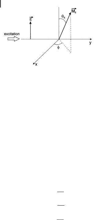
Fig. 5.5. System of coordinates for characterizing the orientation of the emission transition moments.
5.4
Relation between emission anisotropy and angular distribution of the emission transition moments
Let us consider a population of N molecules randomly oriented and excited at time 0 by an infinitely short pulse of light polarized along Oz. At time t, the emission transition moments ME of the excited molecules have a certain angular distribution. The orientation of these transition moments is characterized by yE, the angle with respect to the Oz axis, and by f (azimuth), the angle with respect to the Oz axis (Figure 5.5). The final expression of emission anisotropy should be independent of f because Oz is an axis of symmetry.
For a particular molecule i, the components of the emission transition moments
along the three axes Ox, Oy, Oz are MEaiðtÞ, MEbiðtÞ and MEgiðtÞ, where aiðtÞ, biðtÞ and giðtÞ are the cosines of the angles formed by the emission transition moment
with the three axes (such that ai2bi2gi2 ¼ 1) and ME is the modulus of the vector transition moment.
The total fluorescence intensity at time t is obtained by summing over all molecules emitting at that time. Because there is no phase relation between the elementary emissions, the contributions of each molecule to the intensity components along Ox, Oy and Oz are proportional to the square of its transition moment components along each axis. Summation over all molecules leads to the following expressions for the fluorescence intensity components:
N |
|
IxðtÞ ¼ KME2 Xi 1 ai2ðtÞ ¼ KME2Na2ðtÞ |
|
¼ |
|
N |
|
IyðtÞ ¼ KME2 Xi 1 bi2ðtÞ ¼ KME2Nb2ðtÞ |
ð5:18Þ |
¼ |
|
XN
IzðtÞ ¼ KME2 gi2ðtÞ ¼ KME2Ng2ðtÞ
i¼1