Molecular Fluorescence

For organic molecules, the lifetime of the singlet state ranges from tens of picoseconds to hundreds of nanoseconds, whereas the triplet lifetime is much longer (microseconds to seconds). However, such a di erence cannot be used to make a distinction between fluorescence and phosphorescence because some inorganic compounds (for instance, uranyl ion) or organometallic compounds may have a long lifetime.

Monitoring of phosphorescence or delayed fluorescence enables us to study much slower phenomena. Examples of lifetimes are given in Table 3.1.

3.2.2

Quantum yields

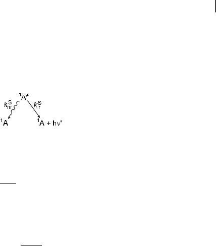
The fluorescence quantum yield FF is the fraction of excited molecules that return to the ground state S0 with emission of fluorescence photons:

In other words, the fluorescence quantum yield is the ratio of the number of emitted photons (over the whole duration of the decay) to the number of absorbed photons. According to Eq. (3.4), the ratio of the d-pulse response iFðtÞ and the number of absorbed photons is given by

and integration of this relation over the whole duration of the decay (mathematically from 0 to infinity) yields FF:

The quantum yields of intersystem crossing ðFiscÞ and phosphorescence ðFPÞ are given by

Using the radiative lifetime, as previously defined, the fluorescence quantum yield can also be written as

48 3 Characteristics of fluorescence emission

It is well known that dioxygen quenches fluorescence (and phosphorescence) (see Chapter 4), but its e ect on quantum yields and lifetimes strongly depends on the nature of the compound and the medium. Oxygen quenching is a collisional process and is therefore di usion-controlled. Consequently, compounds of long lifetime, such as naphthalene and pyrene, are particularly sensitive to the presence of oxygen. Moreover, oxygen quenching is less e cient in media of high viscosity. Oxygen quenching can be avoided by bubbling nitrogen or argon in the solution; however the most e cient method (used particularly in phosphorescence studies) is to perform a number of freeze–pump-thaw cycles.

3.2.3

E ect of temperature

Generally, an increase in temperature results in a decrease in the fluorescence quantum yield and the lifetime because the non-radiative processes related to thermal agitation (collisions with solvent molecules, intramolecular vibrations and rotations, etc.) are more e cient at higher temperatures. Experiments are often in good agreement with the empirical linear variation of lnð1=FF 1Þ versus 1=T.

As mentioned above, phosphorescence is observed only under certain conditions because the triplet states are very e ciently deactivated by collisions with solvent molecules (or oxygen and impurities) because their lifetime is long. These e ects can be reduced and may even disappear when the molecules are in a frozen solvent, or in a rigid matrix (e.g. polymer) at room temperature. The increase in phosphorescence quantum yield by cooling can reach a factor of 103, whereas this factor is generally no larger than 10 or so for fluorescence quantum yield.

In conclusion, lifetimes and quantum yields are characteristics of major importance. Obviously, the larger the fluorescence quantum yield, the easier it is to observe a fluorescent compound, especially a fluorescent probe. It should be emphasized that, in the condensed phase, many parameters can a ect the quantum yields and lifetimes: temperature, pH, polarity, viscosity, hydrogen bonding, presence of quenchers, etc. Attention should be paid to possible erroneous interpretation arising from the simultaneous e ects of several factors (for instance, changes in viscosity due to a variation in temperature).

3.3

Emission and excitation spectra

3.3.1

Steady-state fluorescence intensity

Emission and excitation spectra are recorded using a spectrofluorometer (see Chapter 6). The light source is a lamp emitting a constant photon flow, i.e. a constant amount of photons per unit time, whatever their energy. Let us denote by N0 the constant amount of incident photons entering, during a given time, a unit

503 Characteristics of fluorescence emission

3.3.2

Emission spectra

We have so far considered all emitted photons, whatever their energy. We now focus our attention on the energy distribution of the emitted photons. With this in mind, it is convenient to express the steady-state fluorescence intensity per absorbed photon as a function of the wavelength of the emitted photons, denoted by FlðlFÞ (in m 1 or nm 1) and satisfying the relationship

ðy

0

where FF is the fluorescence quantum yield defined above. FlðlFÞ represents the fluorescence spectrum or emission spectrum: it reflects the distribution of the probability of the various transitions from the lowest vibrational level of S1 to the various vibrational levels of S0. The emission spectrum is characteristic of a given compound.

In practice, the steady-state fluorescence intensity IFðlFÞ measured at wavelength lF (selected by a monochromator with a certain wavelength bandpass DlF) is proportional to FlðlFÞ and to the number of photons absorbed at the excitation wavelength lE (selected by a monochromator). It is convenient to replace this number of photons by the absorbed intensity IAðlEÞ, defined as the di erence between the intensity of the incident light I0ðlEÞ and the intensity of the transmitted light

ITðlEÞ:

The proportionality factor k depends on several parameters, in particular on the optical configuration for observation (i.e. the solid angle through which the instrument collects fluorescence, which is in fact emitted in all directions) and on the bandwidth of the monochromators (i.e. the entrance and exit widths; see Chapter 5).

Furthermore, the intensity of the transmitted light can be expressed using the Beer–Lambert law (see Chapter 2):

where eðlEÞ denotes the molar absorption coe cient of the fluorophore at wavelength lE (in L mol 1 cm 1), l the optical path in the sample (in cm) and c the concentration (in mol L 1). The quantity eðlEÞlc represents the absorbance AðlEÞ at wavelength lE.

52 3 Characteristics of fluorescence emission

low background level whereas in the measurement of low absorbances, two large signals that are slightly di erent are compared. Thanks to outstanding progress in instrumentation, it is now possible in some cases to even detect a single fluorescent molecule (see Chapter 11).

The fluorescence spectrum of a compound may be used in some cases for the identification of species, especially when the spectrum exhibits vibronic bands (e.g. in the case of aromatic hydrocarbons), but the spectra of most fluorescent probes (in the condensed phase) exhibit broad bands.

Equations (3.15)–(3.20) have been written using wavelengths, but they could also have been written using wavenumbers. For example, the integral in Eq. (3.15) is found written in some books (e.g. Birks, 1969, 1973) using wavenumbers instead of wavelengths:

ð0

y

where FnðnFÞ is the fluorescence intensity per unit wavenumber.

Comments should be made here on the theoretical equivalence between Eqs (3.15) and (3.21). The fluorescence quantum yield FF, i.e. the number of photons emitted over the whole fluorescence spectrum divided by the number of absorbed photons, must of course be independent of the representation of the fluorescence spectrum in the wavelength scale (Eq. 3.15) or the wavenumber scale (Eq. 3.21):

ðy ð0

However, as shown in Box 3.3, it should be emphasized that FlðlFÞ is not equal to FnðnFÞ and this has practical consequences.

From the theoretical point of view, the important consequence of Eq. (3.22) is that the conversion of an integral from the wavenumber form to the wavelength form simply consists of replacing FnðnFÞ by FlðlFÞ, and dnF by dlF. However, from the practical point of view, because all spectrofluorometers are equipped with grating monochromators, calculation of the integral must be done with the wavelength form. The fluorescence spectrum is then recorded on a linear wavelength scale at constant wavelength bandpass DlF (which is the integration step) (see Box 3.3).

3.3.3

Excitation spectra

The variations in fluorescence intensity as a function of the excitation wavelength lE for a fixed observation wavelength lF represents the excitation spectrum. According to Eq. (3.20), these variations reflect the evolution of the product I0ðlEÞAðlEÞ. If we can compensate for the wavelength dependence of the incident light (see Chapter 6), the sole term to be taken into consideration is AðlEÞ, which represents the absorption spectrum. The corrected excitation spectrum is thus identical in

3.3 Emission and excitation spectra 53

Box 3.3 Determination of fluorescence quantum yields from fluorescence spectra: wavelength scale or wavenumber scale?

Fluorescence quantum yields are usually determined by integration of the fluorescence spectrum (and subsequent normalization using a standard of known fluorescence quantum yield in order to get rid of the instrumental factor k appearing in Eqs 3.17 or 3.18; see Chapter 6). In practice, attention should be paid to the method of integration.

When the emission monochromator of the spectrofluorometer is set at a certain wavelength lF with a bandpass DlF, the reading is proportional to the number of photons emitted in the wavelength range from lF to lF þ DlF, or in the corresponding wavenumber range from to 1=lF to 1=ðlF þ DlFÞ. The number of detected photons satisfies the relationship:

FlðlFÞDlF ¼ FnðnFÞDnF

where DnF must be positive and is thus defined as 1=lF 1=ðlF þ DlFÞ. Hence,

1

FlðlFÞ ¼ FnðnFÞ lFðlF þ DlFÞ

Because DlF flF, this equation becomes

FlðlFÞlF2 ¼ FnðnFÞ

which clearly shows that FlðlFÞ is not equal to FnðnFÞ.

If a grating monochromator is used to record the fluorescence spectrum, the bandpass DlF is constant and the scale is linear in wavelength. Therefore, after correction of the spectrum (see Chapter 6), the integral should be calculated with the wavelength form (Eq. 3.13). Some workers convert the wavelength scale into the wavenumber scale before integration, but this procedure is incorrect. In some cases, the consequence might be that the quantum yield calculated by comparison with a fluorescent standard is found to be greater than 1!

It should be noted that no such di culty appears with the integral of an absorption spectrum because the absorption coe cient is proportional to the logarithm of a ratio of intensities, so that eðlÞ ¼ eðnÞ. For instance, in the calculation of an oscillator strength (defined in Chapter 2), integration can be done either in the wavelength scale or in the wavenumber scale.

shape to the absorption spectrum, provided that there is a single species in the ground state. In contrast, when several species are present, or when a sole species exists in di erent forms in the ground state (aggregates, complexes, tautomeric forms, etc.), the excitation and absorption spectra are no longer superimposable. Comparison of absorption and emission spectra often provides useful information.

543 Characteristics of fluorescence emission

3.3.4

Stokes shift

The Stokes shift is the gap between the maximum of the first absorption band and the maximum of the fluorescence spectrum (expressed in wavenumbers), Dn ¼ na nf (Figure 3.3).

This important parameter can provide information on the excited states. For instance, when the dipole moment of a fluorescent molecule is higher in the excited state than in the ground state, the Stokes shift increases with solvent polarity. The consequences of this in the estimation of polarity using fluorescent polarity probes is discussed in Chapter 7.

From a practical point of view, the detection of a fluorescent species is of course easier when the Stokes shift is larger.

3.4

E ects of molecular structure on fluorescence

3.4.1

Extent of p-electron system. Nature of the lowest-lying transition

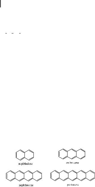
Most fluorescent compounds are aromatic. A few highly unsaturated aliphatic compounds are also fluorescent. Generally speaking, an increase in the extent of the p-electron system (i.e. degree of conjugation) leads to a shift of the absorption and fluorescence spectra to longer wavelengths and to an increase in the fluorescence quantum yield. This simple rule is illustrated by the series of linear aromatic hydrocarbons: naphthalene, anthracene, naphthacene and pentacene emit fluorescence in the ultraviolet, blue, green and red, respectively.

The lowest-lying transitions of aromatic hydrocarbons are of p ! p type, which are characterized by high molar absorption coe cients and relatively high fluorescence quantum yields. When a heteroatom is involved in the p-system, an n ! p transition may be the lowest-lying transition. Such transitions are characterized by molar absorption coe cients that are at least a factor of 102 smaller than those of p ! p transitions. Therefore, according to the Strickler–Berg equation (Section 3.2.1), the radiative lifetime tr is at least 100 times longer than that of low-lying