Molecular Fluorescence

6.2 Time-resolved fluorometry 175

that the probability of detecting two fluorescence pulses per exciting pulse is negligible. Otherwise, the TAC will take into account only the first fluorescence pulse and the counting statistics will be distorted: the decay will appear shorter than it actually is. This e ect is called the ‘pileup e ect’.

The SPT technique o ers several advantages:

. high sensitivity;

.outstanding dynamic range and linearity: three or four decades are common and five is possible;

.well-defined statistics (Poisson distribution) allowing proper weighting of each point in data analysis.

The excitation source is of major importance. Flash lamps running in air, or filled with N2, H2 or D2 are not expensive but the excitation wavelengths are restricted to the 200–400 nm range. They deliver nanosecond pulses, so that decay times of a few hundreds of picoseconds can be measured. Furthermore, the repetition rate is not high (104 –105 Hz) and because the number of fluorescence pulses per exciting pulse must be kept below 5%, the collection period may be quite long, depending on the required accuracy (a few tens of minutes to several hours). For long collection periods, lamp drift may be a serious problem.

Lasers as excitation sources are of course much more e cient and versatile, at the penalty of high cost. Mode-locked lasers (e.g. argon ion lasers) associated with a dye laser or Ti:sapphire laser can generate pulses over a broad wavelength range. The pulse widths are in the picosecond range with a high repetition rate. This rate must be limited to a few MHz in order to let the fluorescence of long lifetime samples vanish before a new exciting pulse is generated.

Synchrotron radiation can also be used as an excitation source with the advantage of almost constant intensity versus wavelength over a very broad range, but the pulse width is in general of the order of hundreds of picosecond or not much less. There are only a few sources of this type in the world.

The time resolution of the instrument is governed not only by the pulse width but also by the electronics and the detector. The linear time response of the TAC is most critical for obtaining accurate fluorescence decays. The response is more linear when the time during which the TAC is in operation and unable to respond to another signal (dead time) is minimized. For this reason, it is better to collect the data in the reverse configuration: the fluorescence pulse acts as the start pulse and the corresponding excitation pulse (delayed by an appropriate delay line) as the stop pulse. In this way, only a small fraction of start pulses result in stop pulses and the collection statistics are better.

Microchannel plate photomultipliers are preferred to standard photomultipliers, but they are much more expensive. They exhibit faster time responses (10to 20fold faster) and do not show a significant ‘color e ect’ (see below).

With mode-locked lasers and microchannel plate photomultipliers, the instrument response in terms of pulse width is 30–40 ps so that decay times as short as 10–20 ps can be measured.

176 6 Principles of steady-state and time-resolved fluorometric techniques

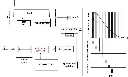
Fig. 6.8. Principle of the stroboscopic technique.

6.2.2.2 Stroboscopic technique

This technique is an interesting alternative to the single-photon timing technique (James et al., 1992). The sample is excited by a train of light pulses delivered by a flash lamp. A computer-controlled digital delay unit is used to gate (or ‘strobe’) the photomultiplier by a voltage pulse (whose width defines a time window) at a time accurately delayed with respect to the light pulse. Synchronization with the flash lamp is achieved by a master clock. By this procedure, only photons emitted from the sample that arrive at the photocathode of the photomultiplier during the gate time will be detected. The fluorescence intensity as a function of time can be constructed by moving the time window after each pulse from before the pulse light to any suitable end time (e.g. ten times the excited-state lifetime). The principle of the stroboscopic technique is shown in Figure 6.8.

The strobe technique o ers some advantages. It does not require expensive electronics. High-frequency light sources are unnecessary because the intensity of the signal is directly proportional to the intensity of the light pulse, in contrast to the single-photon timing technique. High-intensity picosecond lasers operating at low repetition rate can be used, with the advantage of lower cost than cavitydumped, mode-locked picosecond lasers. However, the time resolution of the strobe technique is less than that of the single-photon timing technique, and lifetime measurements with samples of low fluorescence intensity are more di cult.

6.2.2.3 Other techniques

Lifetime instruments using a streak camera as a detector provide a better time resolution than those based on the single-photon timing technique. However, streak cameras are quite expensive. In a streak camera, the photoelectrons emitted

6.2 Time-resolved fluorometry 177

by the photocathode are accelerated into a deflection field. The beam is then swept linearly in time across a microchannel plate electron amplifier that preserves the spatial information. The amplified electron beam is collected by a video camera– computer system. Temporal information is thus converted into spatial information. The time resolution of streak cameras (few picoseconds or less) is better than that of single-photon timing instruments, but the dynamic range is smaller (2–3 decades instead of 3–5 decades).

The instruments that provide the best time resolution (about 100 femtoseconds) are based on fluorescence up-conversion. This very sophisticated and expensive technique will be described in Chapter 11.

6.2.3

Design of phase-modulation fluorometers

Before describing the instruments, it is worth making two preliminary remarks:

(i)The optimum frequency for decay time measurements using either the phase shift or the modulation ratio is, according to Eqs (6.26) and (6.27), such that ot

is close to 1, i.e. f A1=ð2ptÞ. Therefore, for decay times of 10 ps, 1 ns or 100 ns, the optimum frequencies are about 16 GHz, 160 MHz or 1.6 MHz, respectively. These values give an order of magnitude of the frequency ranges that are in principle to be selected depending on the decay times. Figure 6.9 shows simulation data.

(ii)In the case of a single exponential decay, Eqs (6.26) and (6.27) provide two in-

dependent ways of measuring the decay time:

. by phase measurements:

Fig. 6.9. Simulated variations of phase shift and modulation ratio versus frequency using Eqs (6.25) and (6.26).

178 6 Principles of steady-state and time-resolved fluorometric techniques

. by modulation measurements:

The values measured in these two ways should of course be identical and independent of the modulation frequency. This provides two criteria to check whether an instrument is correctly tuned by using a lifetime standard whose fluorescence decay is known to be a single exponential.

Note that the measurement of a decay time is fast (a fraction of a second) for a single exponential decay because a single frequency is su cient. Note also that a significant di erence between the values obtained by means of Eqs (6.35) and (6.36) is compelling evidence of non-exponentiality of the fluorescence decay.

Historically, the first instrument for the determination of lifetime was a phase fluorometer (designed by Gaviola in 1926) operating at a single frequency. Progress in instrumentation enabled variable modulation frequency by employing a cw laser (or a lamp) and an electro-optic modulator (0.1–250 MHz), or by using the harmonic content of a pulsed laser source (up to 2 GHz). These two techniques will now be described.

6.2.3.1 Phase fluorometers using a continuous light source and an electro-optic modulator

The light source can be a xenon lamp associated with a monochromator. The optical configuration should be carefully optimized because the electro-optic modulator (usually a Pockel’s cell) must work with a parallel light beam. The advantages are the low cost of the system and the wide availability of excitation wavelengths. In terms of light intensity and modulation, it is preferable to use a cw laser, which costs less than mode-locked pulsed lasers.

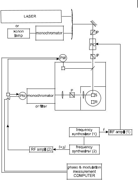
Figure 6.10 shows a multi-frequency phase-modulation fluorometer. A beam splitter reflects a few per cent of the incident light towards a reference photomultiplier (via a cuvette containing a reference scattering solution or not). The fluorescent sample and a reference solution (containing either a scatter or a reference fluorescent compound) are placed in a rotating turret. The emitted fluorescence or scattered light is detected by a photomultiplier through a monochromator or an optical filter. The Pockel’s cell is driven by a frequency synthesizer and the photomultiplier response is modulated by varying the voltage at the second dynode by means of another frequency synthesizer locked in phase with the first one. The two synthesizers provide modulated signals that di er in frequency by a few tens of Hz in order to achieve cross-correlation (heterodyne detection). This procedure is very accurate because the phase and modulation information contained in the signal is transposed to the low-frequency domain where phase shifts and modulation depths can be measured with a much higher accuracy than in the high-frequency domain. For instruments using a cw laser, the standard deviations are currently 0.1–0.2 for the phase shift and 0.002–0.004 for the modulation ratio. When the light source is a xenon lamp, these standard deviations are @0.5 and 0.005, respectively.

180 6 Principles of steady-state and time-resolved fluorometric techniques

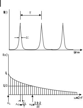
Fig. 6.11. Harmonic content of a pulse train. For a repetition rate of 4 MHz and Dt ¼ 5 ps, oL ¼ 277 GHz, Do ¼ 25:1 MHz.

6.2.3.2 Phase fluorometers using the harmonic content of a pulsed laser

The type of laser source that can be used is exactly the same as for single-photon counting pulse fluorometry (see above). Such a laser system, which delivers pulses in the picosecond range with a repetition rate of a few MHz can be considered as an intrinsically modulated source. The harmonic content of the pulse train – which depends on the width of the pulses (as illustrated in Figure 6.11) – extends to several gigahertz.

For high-frequency measurements, normal photomultipliers are too slow, and microchannel plate photomultipliers are required. However, internal crosscorrelation is not possible with the latter and an external mixing circuit must be used.

The time resolution of a phase fluorometer using the harmonic content of a pulsed laser and a microchannel plate photomultiplier is comparable to that of a single-photon counting instrument using the same kind of laser and detector.

6.2.4

Problems with data collection by pulse and phase-modulation fluorometers

6.2.4.1 Dependence of the instrument response on wavelength. Color e ect

The transit times of photoelectrons in normal photomultipliers depend significantly on the wavelength of the incident photon, whereas this dependence is

182 6 Principles of steady-state and time-resolved fluorometric techniques

is convenient to normalize w2 so that the value is independent of N and the number p of fitted parameters (e.g. for a double-exponential decay, p ¼ 3: two decay times and one pre-exponential factor). Division of w2 by the number of degrees of freedom, n ¼ N p, leads to the reduced chi square wr2 whose value should be close to 1 for a good fit.

In single-photon counting experiments, the statistics obey a Poisson distribution and the expected deviation sðiÞ is approximated to ½RðtiÞ&1=2 so that Eq. (6.38) becomes

In practice, initial guesses of the fitting parameters (e.g. pre-exponential factors and decay times in the case of a multi-exponential decay) are used to calculate the decay curve; the latter is reconvoluted with the instrument response for comparison with the experimental curve. Then, a minimization algorithm (e.g. Marquardt method) is employed to search the parameters giving the best fit. At each step of the iteration procedure, the calculated decay is reconvoluted with the instrument response. Several softwares are commercially available.

6.2.5.2 Phase-modulation fluorometry

The least-squares method is also widely applied to curve fitting in phasemodulation fluorometry; the main di erence with data analysis in pulse fluorometry is that no deconvolution is required: curve fitting is indeed performed in the frequency domain, i.e. directly using the variations of the phase shift F and the modulation ratio M as functions of the modulation frequency. Phase data and modulation data can be analyzed separately or simultaneously. In the latter case the reduced chi squared is given by

where N is the total number of frequencies. In this case, the number of data points is twice the number of frequencies, so that the number of degrees of freedom is n ¼ 2N p.

Data analysis in phase fluorometry requires knowledge of the sine and cosine of the Fourier transforms of the d-pulse response. This of course is not a problem for the most common case of multi-exponential decays (see above), but in some cases the Fourier transforms may not have analytical expressions, and numerical calculations of the relevant integrals are then necessary.

6.2 Time-resolved fluorometry 183

6.2.5.3 Judging the quality of the fit

Once the best fit parameters are obtained, the quality of the fitted decay function must be judged using statistical and graphical criteria.

In the least-squares method, the first criterion is of course the reduced chi squared wr2 (Eqs 6.39 and 6.40), whose value should be close to 1 for a good fit. Acceptable values are in the 0.8–1.2 range. Lower values indicate that the data set is too small for a meaningful fit and higher values are caused by a significant deviation from the theoretical model (e.g. insu cient number of exponential terms). Systematic errors (arising for instance from radiofrequencies interfering with the detection) can also explain higher values.

The values of wr2 in phase-modulation data analysis deserve further comment. Values of the standard deviations, sF and sM, must be assigned; these values are in principle frequency-dependent. At each frequency, a large number of phase shift and modulation measurements is averaged so that values of the standard deviations are easily calculated. However, it is usually the case that when such values are used in the analysis, abnormally high values of wr2 are obtained, which means that values of the standard deviations are underestimated (because of some systematic errors). Therefore, ‘realistic’ frequency-independent values must be assigned. The important consequence is that the value of wr2 is not su cient as a criterion of good fit and that only relative values can be used in accepting or rejecting a theoretical model. For instance, in the case of a multi-exponential decay, when wr2 decreases two-fold or more when an exponential term is added, then addition of this term is justified.

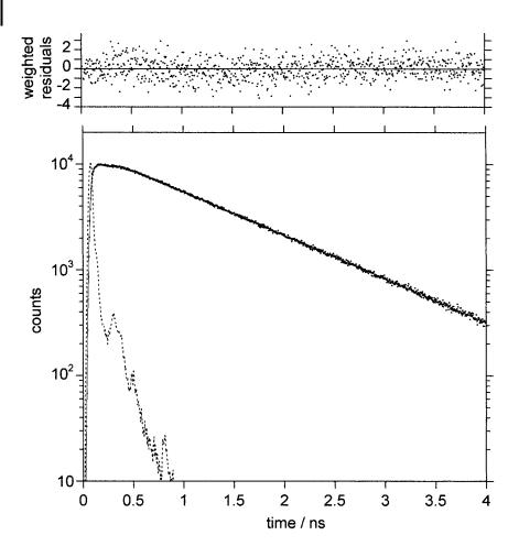
In addition to the value of wr2, graphical tests are useful. The most important of these is the plot of the weighted residuals, defined as

When the number of data points is large (i.e. in the single-photon timing technique, or in phase fluorometry when using a large number of modulation frequencies), the autocorrelation function of the residuals, defined as

is also a useful graphical test of the quality of the fit. Cð jÞ expresses the correlation between the residual in channels j and i þ j. A low-frequency periodicity is symptomatic of radiofrequency interferences. Several other tests (e.g. Durbin–Watson parameter) can also be used (Eaton, 1990).