Molecular Fluorescence

8.1 What is viscosity? Significance at a microscopic level 227

Tab. 8.1. Main fluorescence techniques for the determination of fluidity (from Valeur, 1993)

where k is the Boltzmann constant, T is the absolute temperature and x is the friction coe cient. For translational and rotational di usions, the di usion coefficients are respectively

where r is the hydrodynamic radius of the sphere and V its hydrodynamic volume. In all fluorescence techniques permitting evaluation of the fluidity of a microenvironment by means of a fluorescent probe (see Table 8.1), the underlying physical quantity is a di usion coe cient (either rotational or translational) expressing the viscous drag of the surrounding molecules. The major problem is then to relate the di usion constant D to the viscosity h. This is indeed a di cult problem because Eqs (8.2) and (8.3) are valid only for a rigid sphere that is large compared to the molecular dimensions, moving in a homogeneous Newtonian

228 8 Microviscosity, fluidity, molecular mobility. Estimation by means of fluorescent probes

fluid, and obeying the Stokes hydrodynamic law. Many other relations have been proposed but it should be pointed out that there is no satisfactory relationship between di usion and bulk viscosity for probes. The main reason is that the size of probes is comparable to that of the surrounding molecules forming the microenvironment to be probed. Another di culty arises in the case of organized assemblies such as micellar systems, biological membranes, etc. because the microenvironment is not isotropic.

9 In other words, viscosity is a macroscopic parameter and any attempt to get absolute values of the viscosity of a medium from measurements using a fluorescent probe is hopeless.

The term microviscosity is often used, but again no absolute values can be given, and the best we can do is to speak of an equivalent viscosity, i.e. the viscosity of a homogeneous medium in which the response of the probe is the same. But a difficulty arises as to the choice of the reference solvent because the rotational relaxation rate of a probe in various solvents of the same macroscopic viscosity depends on the nature of the solvent (chemical structure and possible internal order).

Various modifications of the Stokes–Einstein relation have been proposed to take into account the microscopic e ects (shape, free volume, solvent–probe interactions, etc.). In particular, the di usion of molecular probes being more rapid than predicted by the theory, the ‘slip’ boundary condition can be introduced, and sometimes a mixture of ‘stick’ and ‘slip’ boundary conditions is assumed. Equation (8.3) can then be rewritten as

where s is the coupling factor (s ¼ 1 for ‘stick’ and s < 1 for ‘slip’ boundary conditions) and g is the shape factor.

In the case of charged molecules, an additional friction force should be introduced as a result of the induced polarization of the surrounding solvent molecules.

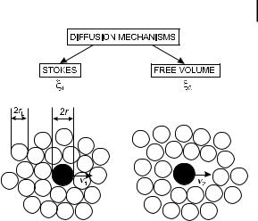
Another microscopic approach to the viscosity problem was developed by Gierer and Wirtz (1953) and it is worthwhile describing the main aspects of this theory, which is of interest because it takes account of the finite thickness of the solvent layers and the existence of holes in the solvent ( free volume). The Stokes–Einstein law can be modified using a microscopic friction coe cient xmicro

A solute molecule moves according to two di usional processes: a viscous process with displacement of solvent molecules (Stokes di usion) and a process associated

8.1 What is viscosity? Significance at a microscopic level 229

Fig. 8.1. Stokes and free volume translational di usion processes. Black circles: solute molecules.

White circles: solvent molecules.

with migration into holes of the solvent ( free volume di usion), as illustrated in Figure 8.1.

The total velocity of the solute molecule is given by v ¼ v1 þ v2. Because the friction coe cient is the ratio of the viscous force to the velocity ðx ¼ F=vÞ, the microscopic friction coe cient xmicro consists of two parts:

x1, corresponding to the Stokes di usional process, can be written as the product of the Stokes friction coe cient multiplied by a correcting factor ft 0 taking into account the finite thickness of the solvent layers

with

where r and rL are the radii of the solute and the solvent molecules, respectively, assuming that they are spherical.

Using Eqs (8.4) to (8.8), the microfriction factor ft for translation is given by

230 8 Microviscosity, fluidity, molecular mobility. Estimation by means of fluorescent probes

For rotational di usion, the correcting factor is

"# 1

The importance of free volume e ects in di usional processes at a molecular level should be further emphasized. An empirical relationship between viscosity and free volume was proposed by Doolittle:

where h0 is a constant, and V0 and Vf are the van der Waals volume and the free volume of the solvent, respectively.

These preliminary considerations should be borne in mind during the following discussion on the various methods of characterization of ‘microviscosity’.

8.2

Use of molecular rotors

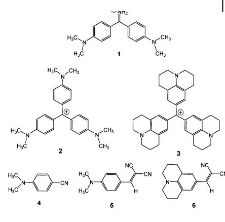
A molecular rotor – as a fluorescent probe – is a molecule that undergoes internal rotation(s) resulting in viscosity-dependent changes in its emissive properties. The possibilities of internal rotation associated with intramolecular charge transfer in various fluorescent molecules have already been examined in Section 3.4.4. In the present section, the viscosity dependence of the fluorescence quantum yield is further discussed, with special attention to the e ect of free volume. Various examples of molecular rotors of practical interest are given in Figure 8.2: they belong to the family of diphenylmethane dyes (e.g. auramine O), triphenylmethane dyes (e.g. crystal violet), and TICT compounds that can form, upon excitation, a twisted intramolecular charge transfer state (e.g. DMABN) (the latter compounds possess an electron-donating group (e.g. dimethylamino group) conjugated to an electronwithdrawing group (e.g. cyano group)).

In solvents of medium and high viscosity, an empirical relation has been proposed (Loutfy and Arnold, 1982) to link the non-radiative rate constant for deexcitation to the ratio of the van der Waals volume to the free volume according to

where knr0 is the free-rotor reorientation rate and x is a constant for a particular probe. Because the fluorescence quantum yield is related to the radiative and non-

8.2 Use of molecular rotors 231

Fig. 8.2. Examples of molecular rotors. 1: auramine O. 2: crystal violet. 4: p-N,N-dimethylaminobenzonitrile (DMABN). 5: p-N,N-dimethylaminobenzylidenemalononitrile. 6: julolidinebenzylidenemalononitrile.

radiative rate constants by the expression FF ¼ kr=ðkr þ knrÞ, we obtain

For small fluorescence quantum yields, an approximate expression can be used:

232 8 Microviscosity, fluidity, molecular mobility. Estimation by means of fluorescent probes

When changes in viscosity are achieved by variations of temperature, this expression should be rewritten as

In most investigations in solvents of medium or high viscosity, or in polymers above the glass transition temperature, the fluorescence quantum yields were in fact found to be a power function of the bulk viscosity, with values of the exponent x less than 1 (e.g. for p-N,N-dimethylaminobenzylidenemalononitrile, x ¼ 0:69 in glycerol and 0.43 in dimethylphthalate). This means that the e ective viscosity probed by a molecular rotor appears to be less than the bulk viscosity h because of free volume e ects.

Molecular rotors allow us to study changes in free volume of polymers as a function of polymerization reaction parameters, molecular weight, stereoregularity, crosslinking, polymer chain relaxation and flexibility. Application to monitoring of polymerization reactions is illustrated in Box 8.1.

8.3

Methods based on intermolecular quenching or intermolecular excimer formation

Dynamic quenching of fluorescence is described in Section 4.2.2. This translational di usion process is viscosity-dependent and is thus expected to provide information on the fluidity of a microenvironment, but it must occur in a time-scale comparable to the excited-state lifetime of the fluorophore (experimental time window). When transient e ects are negligible, the rate constant kq for quenching can be easily determined by measuring the fluorescence intensity or lifetime as a function of the quencher concentration; the results can be analyzed using the Stern–Volmer relation:

where F0 and F are the fluorescence quantum yields of the probe in the absence and in the presence of quencher, respectively.

Let us recall that, if the bimolecular process is di usion-controlled, kq is identical to the di usional rate constant k1. If k1 is assumed to be independent of time (see Chapter 4), it can be expressed by the following simplified form (Smoluchowski relation):

where Rc is the distance of closest approach (in cm), D is the mutual di usion co- e cient (in cm2 s 1), N is equal to Na=1000, Na being Avogadro’s number. The distance of closest approach is generally taken as the sum of the radii of the two

8.3 Methods based on intermolecular quenching or intermolecular excimer formation 233

Box 8.1 Monitoring of polymerization reactions by means of molecular rotorsa)

The variations in fluorescence intensity of compound 1 during the polymerization reaction of methyl methacrylate (MMA), ethyl methacrylate (EMA) and n- butyl methacrylate (n-BMA), initiated using AIBN at 70 C, are shown in Figure B8.1.1.

At the beginning of the polymerization reaction, the viscosity of the medium is low, and e cient rotation (about the ethylenic double bond and the single bond linking ethylene to the phenyl ring) accounts for the low fluorescence quantum yield. After a lag period, when approaching the polymer glassy state, the fluorescence intensity increases rapidly as a result of the sharp increase in

Fig. B8.1.1. Variation in the fluorescence intensity of compound 1 during the polymerization of methyl methacrylate (MMA), ethyl methacrylate (EMA), n-butyl methacrylate (n-BMA) (reproduced with permission from Louftya)).

234 8 Microviscosity, fluidity, molecular mobility. Estimation by means of fluorescent probes

viscosity with drastic reduction of the free volume. Then, the fluorescence intensity levels o when the limiting conversion is reached.

It should be noted that the rate of change of fluorescence intensity and the fluorescence enhancement factor depend on the polymerization conditions (temperature, initiator concentration, monomer reactivity) and on the nature of the polymer formed.

Such an easy way to monitor on-line the progress of bulk polymerization, in order to prevent runaway reactions, is of great practical interest.

a)Loufty R. O. (1986) Pure & Appl. Chem. 58, 1239.

molecules (RM for the fluorophore and RQ for the quencher). The mutual di usion coe cient D is the sum of the translational di usion coe cients of the two species, DM and DQ.

The method using intermolecular excimer formation is based on the same principle because this process is also di usion-controlled. Excimers should, of course, be formed during the monomer excited-state lifetime. In Section 4.4.1, it was shown that the ratio IE=IM of the intensities of the excimer and monomer bands is proportional to k1 provided that the transient term can be neglected. When the dissociation rate of the excimer is slow with respect to de-excitation, the rela-

where tE is the excimer lifetime, and kr and kr0 are the radiative rate constants of the monomer and excimer, respectively. It should be emphasized that erroneous conclusions may be drawn as to the changes in fluidity of the host matrix as a function of temperature if the excimer lifetime tE is not constant over the range of temperature investigated. Time-resolved fluorescence experiments are then required. The relevant equations are given in Chapter 4 (Eqs 4.43–4.47).

Changes in fluidity of a medium can thus be monitored via the variations of I0=I 1 for quenching, and IE=IM for excimer formation, because these two quantities are proportional to the di usional rate constant k1, i.e. proportional to the di usion coe cient D. Once again, we should not calculate the viscosity value from D by means of the Stokes–Einstein relation (see Section 8.1).

The serious drawback of the methods of evaluation of fluidity based on intermolecular quenching or excimer formation is that the translational di usion can be perturbed in constrained media. It should be emphasized that, in the case of biological membranes, problems in the estimation of fluidity arise from the presence of proteins and possible additives (e.g. cholesterol). Nevertheless, excimer formation with pyrene or pyrene-labeled phospholipids can provide interesting in-