Molecular Fluorescence

Scheme 7.1, relevant to an amphiprotonic solvent). Using Eq. (7.2), the multiple linear regression equation for the fluorescence maximum (expressed in 103 cm 1) is

nfmax ¼ 26:71 2:02p 1:58a 1:32b

with a very good correlation coe cient (r ¼ 0:997).

It should be noted that 4-amino-7-methyl-coumarin undergoes photoinduced charge transfer (see Section 7.3) from the amino group to the carbonyl group. Therefore, in the excited state, the hydrogen bonds involving the more negatively charged oxygen and the more positively charged amino group are stronger than in

Scheme 7.1

7.3 Photoinduced charge transfer (PCT) and solvent relaxation 207

the solute is short with respect to the excited-state lifetime, fluorescence will essentially be emitted from molecules in equilibrium with their solvation shell (F0 in Figure 7.2). Emission of a fluorescence photon being quasi-instantaneous, the solute recovers its ground state dipole moment and a new relaxation process leads to the most stable initial configuration of the system solute–solvent in the ground state.

In contrast, if the medium is too viscous to allow solvent molecules to reorganize, emission arises from a state close to the Franck–Condon state (FC) (as in the case of a nonpolar medium) and no shift of the fluorescence spectrum will be observed (F in Figure 7.2).

Finally, if the solvent reorganization time is of the order of the excited-state lifetime, the first emitted photons will correspond to wavelengths shorter than those emitting at longer times. In this case, the fluorescence spectrum observed under continuous illumination will be shifted but the position of the maximum cannot be directly related to the solvent polarity.

It should be recalled that, in polar rigid media, excitation on the red-edge of the absorption spectrum causes a red-shift of the fluorescence spectrum with respect to that observed on excitation in the bulk of the absorption spectrum (see the explanation of the red-edge e ect in Section 3.5.1). Such a red-shift is still observable if the solvent relaxation competes with the fluorescence decay, but it disappears in fluid solutions because of dynamic equilibrium among the various solvation sites.

It is expected that, during the reorganization of solvent molecules, the time evolution of the fluorescence intensity depends on the observation wavelength, but once the equilibrium solute–solvent configuration is attained, the fluorescence decay only reflects the depopulation of the excited state. From the time-resolved fluorescence intensities recorded at various wavelengths, the fluorescence spectrum at a given time can be reconstructed, so that the time evolution of the fluorescence spectrum can be monitored during solvent relaxation. Fluorescence thus provides an outstanding tool for monitoring the response time of solvent molecules (or polar molecules of a microenvironment) following excitation of a probe molecule whose dipole moment is quasi-instantaneously changed by absorption of a photon.

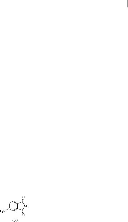
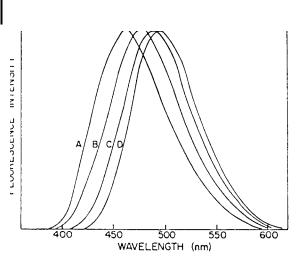
The principle of the determination of time-resolved fluorescence spectra is described in Section 6.2.8. For solvent relaxation in the nanosecond time range, the single-photon timing technique can be used. The first investigation using this technique was reported by Ware and coworkers (1971). Figure 7.3 shows the reconstructed spectra of 4-aminophthalimide (4-AP) at various times after excitation. The solvent, propanol at 70 C, is viscous enough to permit observation of solvent relaxation in a time range compatible with the instrument response (FWHM of 5 ns).

208 7 Effect of polarity on fluorescence emission. Polarity probes

Fig. 7.3. Time-resolved fluorescence spectrum of 4- aminophthalimide at 70 C in n-propanol. A: 4 ns; B: 8 ns; C: 15 ns; D: 23 ns (from Ware, 1971).

The shift of the fluorescence spectrum as a function of time reflects the reorganization of propanol molecules around the excited phthalimide molecules, whose dipole moment is 7.1 D instead of 3.5 D in the ground state (with a change in orientation of 20 ). The time evolution of this shift is not strictly a single exponential.

In contrast, at room temperature, the reconstructed fluorescence spectra were found to be identical to the steady-state spectrum, which means that solvent relaxation occurs at times much shorter than 1 ns in fluid solution.

From a practical point of view, it should be emphasized that, if relaxation is not complete within the excited-state lifetime, this can lead to misinterpretation of the shift of the steady-state fluorescence spectrum in terms of polarity.

The technique of fluorescence up-conversion (see Chapter 11), allowing observations at the time-scale of picoseconds and femtoseconds, prompted a number of fundamental investigations on solvation dynamics that turned out to be quite complex (Barbara and Jarzeba, 1990) (see Box 7.1).

7.4

Theory of solvatochromic shifts

If solvent (or environment) relaxation is complete, equations for the dipole–dipole interaction solvatochromic shifts can be derived within the simple model of spherical-centered dipoles in isotropically polarizable spheres and within the assumption of equal dipole moments in Franck–Condon and relaxed states. The solvatochromic shifts (expressed in wavenumbers) are then given by Eqs (7.3) and (7.4) for absorption and emission, respectively:

7.4 Theory of solvatochromic shifts 209

Box 7.1 Solvation dynamics

To understand solvation dynamics, it is necessary to recall some aspects of dielectric relaxation in the framework of the simple continuum model, which treats the solvent as a uniform dielectric medium with exponential dielectric response.

When a constant electric field is suddenly applied to an ensemble of polar molecules, the orientation polarization increases exponentially with a time constant tD called the dielectric relaxation time or Debye relaxation time. The reciprocal of tD characterizes the rate at which the dipole moments of molecules orient themselves with respect to the electric field.

A single Debye relaxation time tD has been measured for a number of common liquids, called Debye liquids. However, for alcohols, three relaxation times (tD1 > tD2 > tD3) are generally found:

. tD1 is relevant to the dynamics of hydrogen bonds (formation and breaking) in aggregates of alcohol molecules;

. tD2 corresponds to the rotation of single alcohol molecules;

. tD3 is assigned to the rotation of the hydroxyl group around the CaO bond.

For example, for ethanol at room temperature tD1 ¼ 191 ps, tD2 ¼ 16 ps, tD3 ¼ 1:6 ps.

Consequently, the time evolution of the center gravity (expressed in wavenumbers) of the fluorescence spectrum of a fluorophore in a polar environment should be written in the following general form:

X

nðtÞ ¼ nðyÞ þ ðnð0Þ nðyÞÞ ai expð t=tSi Þ

i

where nð0Þ, nðtÞ and nðyÞ respectively are the wavenumbers of the center of gravity immediately after excitation, at a certain time t after excitation, and at a time su ciently long to ensure the excited-state solvent configuration is at equilibrium. tSi represents the spectral relaxation times and Pai ¼ 1.

i

From the above equation it appears convenient to characterize solvation dynamics by means of the solvation time correlation function CðtÞ, defined asa)

CðtÞ ¼ nðtÞ nðyÞ nð0Þ nðyÞ

This function varies from 1 to 0 as time varies from 0 (instant of excitation) to y (i.e. when the equilibrium solute–solvent interaction is attained). It is assumed that (i) the fluorescence spectrum is shifted without change in shape, (ii) there is no contribution of vibrational relaxation or changes in geometry to the

212 7 Effect of polarity on fluorescence emission. Polarity probes

bonding donor or acceptor capability, a linear behavior is often observed, which allows us to determine the increase in dipole moment Dmge upon excitation, provided that a correct estimation of the cavity radius is possible. The uncertainty arises from estimation of the Onsager cavity and from the assumption of a spherical shape of this cavity. For elongated molecules, an ellipsoid form is more appropriate. In spite of these uncertainties, the Lippert–Mataga relation is widely used by taking the molecular radius as the cavity radius. Furthermore, Suppan (1983) derived another useful equation from Eqs (7.3) and (7.4) under the assumption that mg and me are colinear but without any assumption about the cavity radius a or the form of the solvent polarity function. This equation involves the di erences in absorption and emission solvatochromic shifts between two solvents 1 and 2:

Equations (7.6) and (7.7) provide a means of determining excited dipole moments together with dipole vector angles, but they are valid only if (i) the dipole moments in the FC and relaxed states are identical, (ii) the cavity radius remains unchanged upon excitation, (iii) the solvent shifts are measured in solvents of the same refractive index but of di erent dielectric constants.

When the emissive state is a charge transfer state that is not attainable by direct excitation (e.g. which results from electron transfer in a donor–bridge–acceptor molecule; see example at the end of the next section), the theories described above cannot be applied because the absorption spectrum of the charge transfer state is not known. Weller’s theory for exciplexes is then more appropriate and only deals with the shift of the fluorescence spectrum, which is given by

When a twisted intramolecular charge transfer (TICT) state is formed in the excited state (see Section 3.4.4 for the description of TICT formation), the molecular geometry and the charge distribution must be taken into account. Neglecting the ground state dipole moment with respect to that of the excited state and approximating the solute polarizability to a3=2, the following formula is obtained (Rettig, 1982):

7.5 Examples of PCT fluorescent probes for polarity 213

Tab. 7.3. Ground state and excited state dipole moments of some fluorophores determined from solvatochromic shifts (except data from reference 6)

a)4-N,N-dimethylamino-40-nitrostilbene

b)4-N,N-dimethylaminobenzonitrile

c)6-propionyl-2-(dimethylaminonaphthalene)

d)4-dicyanomethylene-2-methyl-6-p-dimethylamino-styryl-4H-pyran

1)Suppan P. (1987) J. Chem. Soc., Faraday Trans. 1 83, 495.

2)Hagan T., Pilloud D. and Suppan P. (1987) Chem. Phys. Lett. 139, 499.

3)Suppan P. (1985) J. Lumin. 33, 29.

4)Baumann W. and Nagy Z. (1993) Pure Appl. Chem. 65, 1729.

5)Catalan J., Perez P., Laynez J. and Blanco F. G. (1991) J. Fluorescence 1, 215.

6)Samanta A. and Fessenden R. W. (2000) J. Phys. Chem. A 104, 8972.

7)Meyer M. and Mialocq J. C. (1985) Opt. Commun. 64, 264.

The assumptions made in theories of solvatochromic shifts, together with the uncertainty over the size and shape of the cavity radius, explain why the determination of excited-state dipole moments is not accurate. Examples of values of excited state dipole moments are given in Table 7.3.

7.5

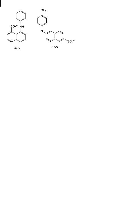
Examples of PCT fluorescent probes for polarity

One of the most well known polarity probes is ANS (1-anilino-8-naphthalene sulfonate), discovered by Weber and Lawrence in 1954. It exhibits the interesting feature of being non-fluorescent in aqueous solutions and highly fluorescent in solvents of low polarity. This feature allows us to visualize only hydrophobic regions of biological systems without interference from non-fluorescent ANS molecules remaining in the surrounding aqueous environment.