Molecular Fluorescence

186 6 Principles of steady-state and time-resolved fluorometric techniques

less closely spaced time constants means that the number of fitting parameters is large enough – considering the limited accuracy of the experimental data – but it does not prove that the number of components is two (or three, or four), unless it is already known that the system can be described by a physical model involving distinct exponentials.

In some circumstances, it can be anticipated that continuous lifetime distributions would best account for the observed phenomena. Examples can be found in biological systems such as proteins, micellar systems and vesicles or membranes. If an a priori choice of the shape of the distribution (i.e. Gaussian, sum of two Gaussians, Lorentzian, sum of two Lorentzians, etc.) is made, a satisfactory fit of the experimental data will only indicate that the assumed distribution is compatible with the experimental data, but it will not demonstrate that this distribution is the only possible one, and that a sum of a few distinct exponentials should be rejected.

To answer the question as to whether the fluorescence decay consists of a few distinct exponentials or should be interpreted in terms of a continuous distribution, it is advantageous to use an approach without a priori assumption of the shape of the distribution. In particular, the maximum entropy method (MEM) is capable of handling both continuous and discrete lifetime distributions in a single analysis of data obtained from pulse fluorometry or phase-modulation fluorometry (Brochon, 1994) (see Box 6.1).

6.2.6

Lifetime standards

The excited-state lifetimes of some compounds that can be used as standards are given in Table 6.2. These values are the averages of data obtained from eight laboratories. There is some deviation from one laboratory to another. For instance, the values reported for POPOP in deoxygenated cyclohexane range from 1.07 to 1.18 ns. The unavoidable small artefacts of any instrument, the di erent origins of the samples and solvents, the di culty of preparing identical solutions without any trace of impurity, quencher, etc., can explain the small deviations observed from laboratory to laboratory. However, more important than the lifetime value itself, is the control that the instrument is properly tuned. After selecting one of the standards in Table 6.1 whose characteristics (lifetime, excitation and observation wavelengths) are preferentially not very di erent from those of the sample to be studied, it is advisable to check that this selected standard indeed exhibits a single exponential decay with a value consistent with that reported in Table 6.2. In the case of short lifetime measurements requiring deconvolution, it should be checked that the reconvoluted curve satisfactorily superimposes the experimental curve, especially in the rise part of the curve.

When normal photomultipliers that exhibit a ‘color e ect’ (see above) are used, the compounds of Table 6.2 that have a short lifetime (e.g. POPOP, PPO) can be used in place of a scattering solution in order to remove this e ect (this method is valid for both pulse and phase fluorometries). Such a reference fluorophore must

6.2 Time-resolved fluorometry 187

Box 6.1 The maximum entropy method (MEM)

The maximum entropy method has been successfully applied to pulse fluorometry and phase-modulation fluorometrya–e). Let us first consider pulse fluorometry. For a multi-exponential decay with n components whose fractional amplitudes are ai, the d-pulse response is

Xn

IðtÞ ¼ ai expð t=tiÞ

i¼1

or, for a distribution of decay times,

ð

IðtÞ ¼ aðtÞ expð t=tÞ dt

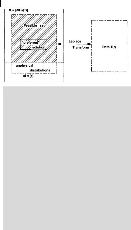
The problem is to determine the spectrum of decay times aðtÞ from timeresolved fluorescence data. aðtÞ appears as the inverse Laplace transform of the fluorescence decay deconvolved by the light pulse. However, inverting the Laplace transform is very ill-conditioned. Consequently, the unavoidable small errors in the measurement of the fluorescence decay or light pulse profile can lead to very large changes in the reconstruction of aðtÞ, i.e. a large multiplicity of allowable solutions. Among these solutions that fit equally well the experimental decay on the basis of statistical tests (mainly chi-squared values, weighted residuals and autocorrelation functions), some of them can be rejected when they contain unphysical features. The remaining set of solutions is called the feasible set (Figure B6.1.1) from which we must choose one member.

The choice of the preferred solution within the feasible set can be achieved by maximizing some function F½aðtÞ& of the spectrum that introduces the fewest artefacts into the distribution. It has been proved that only the Shannon–Jaynes entropy S will give the least correlated solutionf ). All other maximization (or regularization) functions introduce correlations into the solution not demanded by the data. The function S is defined as

where m is the model that encodes our prior knowledge about the system. It has been shown that if we have no knowledge of which values of the fractional amplitudes a are expected, they all have equal prior probability, and m is a flat distribution (mi ¼ constant).

In phase-modulation fluorometry, it is convenient to use the fractional contributions fi instead of the fractional amplitudes, as shown in Eqs (6.30) and (6.31). The above equation is thus rewritten as

6.2 Time-resolved fluorometry 189

Ð

(with mðtÞ dt ¼ 1 if no prior knowledge of the distribution).

The commercially available software (Maximum Entropy Data Consultant Ltd, Cambridge, UK) allows reconstruction of the distribution aðtÞ (or f ðtÞ) which has the maximal entropy S subject to the constraint of the chi-squared value. The quantified version of this software has a full Bayesian approach and includes a precise statement of the accuracy of quantities of interest, i.e. position, surface and broadness of peaks in the distribution. The distributions are recovered by using an automatic stopping criterion for successive iterates, which is based on a Gaussian approximation of the likelihood.

An example of recovered distribution is shown in Figure B6.1.2. It concerns the distribution of lifetimes of 2,6-ANS solubilized in the outer core region of sodium dodecylsulfate micellesg). In fact, the microheterogeneity of solubilized sites results in a distribution of lifetimes.

be excitable and observable under the same conditions as those of the sample. However, it should be emphasized that the lifetime value of the reference fluorophore must not be taken from Table 6.2 (because the value may slightly di er from one instrument to another), but be measured on the same instrument and under the same conditions as those of the investigations on new samples to be done using this reference fluorophore.

It is interesting to note that when using two fluorophores (whose fluorescence decays are known to be single exponentials), one as a sample and the other as a reference, it is possible to determine the lifetimes of both the fluorophores without external reference: this can be achieved in data analysis by varying the reference lifetime until a minimum value of wr2 is reached.

6.2.7

Time-dependent anisotropy measurements

6.2.7.1 Pulse fluorometry

The time dependence of emission anisotropy is defined as (see Chapter 5):

1906 Principles of steady-state and time-resolved fluorometric techniques

Tab. 6.2. Lifetime of various compounds in deoxygenated fluid solutions at 20 C. Averages of

the values measured by eight laboratories by either pulse fluorometry (four laboratories) or phase fluorometry (four laboratories)a)

a)Data collected by N. Boens and M. Ameloot.

b)Abbreviations used: NATA: N-acetyl-L-tryptophanamide, DPA: 9,10diphenylanthracene, POPOP: 1,4-bis(5-phenyloxazol-2-yl)benzene, PPO: 2,5-diphenyloxazole, SPA: N-(3-sulfopropyl)acridinium. All solutions are deoxygenated by repetitive freeze–pump–thaw cycles or by bubbling N2 or Ar through the solutions.

c)The quoted errors are sample standard deviations s

d)Number of lifetime data measured.

e)Number of lifetime data used in the calculation of the mean lifetime t and its standard deviation s. The di erence between columns d and e gives the number of outliers.

where IkðtÞ and I?ðtÞ are the polarized components parallel and perpendicular to the direction of polarization of the incident light, and IðtÞ is the total fluorescence intensity.

For a homogeneous population of fluorophores, i.e. for fluorophores characterized by the same decay of IðtÞ and the same rðtÞ, the polarized components are

192 6 Principles of steady-state and time-resolved fluorometric techniques

6.2.7.2Phase-modulation fluorometry

Instead of recording separately the decays of the two polarized components, we measure the di erential polarized phase angle DðoÞ ¼ F F? between these two components and the polarized modulation ratio LðoÞ ¼ m=m?. It is interesting to define the frequency-dependent anisotropy as follows:

At low frequency, rðoÞ tends towards the steady-state anisotropy, and at high frequency rðoÞ approaches r0, the emission anisotropy in the absence of rotational motions.

The following relationships are used for data analysis:

where Pk and Qk are the sine and cosine transforms of IðtÞ, and P? and Q? are the sine and cosine transforms of I?ðtÞ.

6.2.8

Time-resolved fluorescence spectra

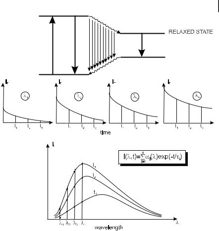
Evolution of fluorescence spectra during the lifetime of the excited state can provide interesting information. Such an evolution occurs when a fluorescent compound is excited and then evolves towards a new configuration whose fluorescent decay is di erent. A typical example is the solvent relaxation around an excitedstate compound whose dipole moment is higher in the excited state than in the ground state (see Chapter 7): the relaxation results in a gradual red-shift of the fluorescence spectrum, and information on the polarity of the microenvironment around a fluorophore is thus obtained (e.g. in biological macromolecules).

Figure 6.14 shows how the fluorescence spectra at various times are recovered from the fluorescence decays at several wavelengths. The principle of the measurements is di erent in pulse and in phase fluorometry.

194 6 Principles of steady-state and time-resolved fluorometric techniques

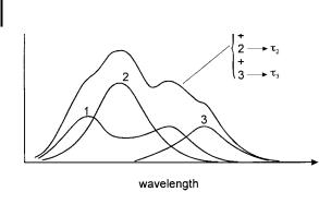
Fig. 6.15. Decomposition of a fluorescence spectrum into its components.

6.2.9

Lifetime-based decomposition of spectra

A fluorescence spectrum may result from overlapping spectra of several fluorescent species (or several forms of a fluorescent species). If each of them is characterized by a single lifetime, it is possible to decompose the overall spectrum into its components.

Let us consider for instance a spectrum consisting of three components whose lifetimes, t1; t2; t3; . . . have been determined separately (Figure 6.15).

Decomposition of the fluorescence spectrum is possible in pulse fluorometry by analyzing the decay with a three-exponential function at each wavelength

P

i¼1

The procedure in phase-modulation fluorometry is more straightforward. The sine and cosine Fourier transforms of the d-pulse response are, according to Eqs (6.30) and (6.31), given by