Molecular Fluorescence

4.6 Excitation energy transfer 115

Box 4.4 Energy of interaction between a donor molecule and an acceptor molecule

Considering that only two electrons are involved in a transition, one on D and one on A, the properly antisymmetrized wavefunctions for the initial excited state Ci (D excited but not A) and the final excited state Cf (A excited but not D) can be written as

1

Ci ¼ p ðCD ð1ÞCAð2Þ CD ð2ÞCAð1ÞÞ

2

ðB4:4:1Þ

1

Cf ¼ p ðCDð1ÞCA ð2Þ CDð2ÞCA ð1ÞÞ

2

where the numbers 1 and 2 refer to the two electrons involved.

The interaction matrix element describing the coupling between the initial and final states is given by

U ¼ hCD ð1ÞCAð2ÞjVjCDð1ÞCA ð2Þi hCD ð1ÞCAð2ÞjVjCDð2ÞCA ð1Þi

ðB4:4:3Þ

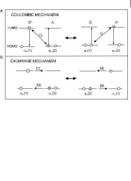
In the first term, Uc, usually called the Coulombic term, the initially excited electron on D returns to the ground state orbital while an electron on A is simultaneously promoted to the excited state. In the second term, called the exchange term, Uex, there is an exchange of two electrons on D and A. The exchange interaction is a quantum-mechanical e ect arising from the symmetry properties of the wavefunctions with respect to exchange of spin and space coordinates of two electrons.

The Coulombic term can be expanded into a sum of terms (multipole– multipole series), but it is generally approximated by the first predominant term representing the dipole–dipole interaction between the transition dipole moments MD and MA of the transitions D ! D and A ! A (the squares of the transition dipole moments are proportional to the oscillator strengths of these transitions):

where r is the donor–acceptor separation. This expression can be rewritten as:

116 4 Effects of intermolecular photophysical processes on fluorescence emission

in which Udd is expressed in cm 1, the transition moments in Debye (1 Debye unit ¼ 3:33 10 30 Coulomb meter), and r in nanometers. yDA is the angle between the two transition moments and yD and yA are the angles between each transition moment and the vector connecting them.

The magnitude of this term can be large even at long distances (up to 80– 100 A˚ ) if the two transitions on D and A are allowed. The excitation energy is transferred through space.

The dipole approximation is valid only for point dipoles, i.e. when the donor– acceptor separation is much larger than the molecular dimensions. At short distances or when the dipole moments are large, it should be replaced by a monopole–monopole expansion. Higher multipole terms should also be included in the calculations.

The exchange term represents the electrostatic interaction between the charge clouds. The transfer in fact occurs via overlap of the electron clouds and requires physical contact between D and A. The interaction is short range because the electron density falls o approximately exponentially outside the boundaries of the molecules. For two electrons separated by a distance r12 in the pair DaA, the space part of the exchange interaction can be written as

where FA and FD are the contributions of the spatial wavefunction to the total wavefunctions CA and CD that include the spin functions. The spin selection rules (Wigner’s rules) for allowed energy transfer are obtained by integration over the spin coordinates.

The transfer rate kT is given by Fermi’s Golden Rule:

where r is a measure of the density of the interacting initial and final states, as determined by the Franck–Condon factors, and is related to the overlap integral between the emission spectrum of the donor and the absorption spectrum of the acceptor.

By substituting Eq. (B4.4.5) into Eq. (B4.4.7), we obtain the Fo¨rster rate constant kTdd (Eq. 4.78 in the text) for energy transfer in the case of long-range dipole–dipole interaction, and substitution of Eq. (B4.4.6) into Eq. (B4.4.7) leads to the Dexter rate constant kexT (Eq. 4.85 in the text) for the short-range exchange interaction.

4.6 Excitation energy transfer 117

Fig. 4.14. Schematic representation of the (A) Coulombic and

(B) exchange mechanisms of excitation energy transfer. CI: Coulombic interaction; EE: electron exchange.

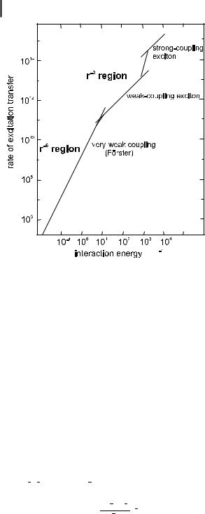
Fig. 4.15. Distinction between strong, weak and very weak coupling.

Strong coupling (U gDE, U gDw, De) The coupling is called strong if the intermolecular interaction is much larger than the interaction between the electronic and nuclear motions within the individual molecules. In this case, the Coulombic term Uc is much larger than the width of the individual transitions D ! D and A ! A . Then, all the vibronic subtransitions in both molecules are virtually at resonance with one another.

118 4 Effects of intermolecular photophysical processes on fluorescence emission

Strongly coupled systems are characterized by large di erences between their absorption spectra and those of their components. For a two-component system, two new absorption bands are observed due to transitions of the in-phase and out- of-phase combinations of the locally excited states. These two transitions are separated in energy by 2jUj.

In the strong coupling case, the transfer of excitation energy is faster than the nuclear vibrations and the vibrational relaxation (@10 12 s). The excitation energy is not localized on one of the molecules but is truly delocalized over the two components (or more in multi-chromophoric systems). The transfer of excitation is a coherent process9); the excitation oscillates back and forth between D and A and is never more than instantaneously localized on either molecule. Such a delocalization is described in the frame of the exciton theory10).

A rate of transfer can be defined as the reciprocal of the time required for the excitation, initially localized on D, to reach a maximum density on A. The rate constant is

where h is Planck’s constant. When U is approximated by a dipole–dipole interaction, the distance dependence of U, and consequently of kT, is r 3 (see Eq. B4.4.5 in Box 4.4). It is important to note that, in contrast, the dependence is r 6 in the case of very weak coupling (see below).

Weak coupling (U gDE, Dw gU gDe) The interaction energy is much lower than the absorption bandwidth but larger than the width of an isolated vibronic level. The electronic excitation in this case is more localized than under strong coupling. Nevertheless, the vibronic excitation is still to be considered as delocalized so that the system can be described in terms of stationary vibronic exciton states.

Weak coupling leads to minor alterations of the absorption spectrum (hypochromism or hyperchromism, Davidov splitting of certain vibronic bands).

The transfer rate is fast compared to vibrational relaxation but slower than nuclear motions, in contrast to the strong coupling case. It can be approximated as

where Svw is the vibrational overlap integral of the intramolecular transition v $ w. This is the transfer rate between an excited molecule with the vibrational quantum number v and an unexcited one with the quantum number w. Because Svw < 1, the

4.6 Excitation energy transfer 119

transfer rate is slower than in the case of strong coupling. The term USvw2 represents the interaction energy between the involved vibronic transitions.

Very weak coupling (U fDe fDw) The interaction energy is much lower than the vibronic bandwidth. Because the coupling is less than in the preceding cases, the condition for resonance becomes more and more stringent. However, the vibronic bandwidths are generally broadened by thermal and solvent e ects (the absorption bands are in fact broad in fluid solutions) so that energy transfer in the very weak coupling limit turns out to be very general.

In this case, there is little or no alteration of the absorption spectra. The vibrational relaxation occurs before the transfer takes place. The transfer rate is given by

This expression shows that the transfer rate depends on the square of the interaction energy11). For dipole–dipole interaction, the distance dependence is thus r 6 instead of r 3 for the preceding cases.

Figure 4.16 shows the rates of energy transfer in the three coupling cases. There is some ambiguity in defining a transfer rate in the cases of strong and weak couplings because of more or less delocalized excitation. It is only in the case of very weak coupling that a transfer rate can be defined unequivocally.

Fo¨rster’s formulation of long-range dipole–dipole transfer (very weak coupling) Fo¨r- ster derived the following expression for the transfer rate constant from classical considerations as well as on quantum-mechanical grounds:

where kD is the emission rate constant of the donor and tD0 its lifetime in the absence of transfer, r is the distance between the donor and the acceptor (which is assumed to remain unchanged during the lifetime of the donor), and R0 is the critical distance or Fo¨rster radius, i.e. the distance at which transfer and spontaneous decay of the excited donor are equally probable ðkT ¼ kDÞ. The characteristic inverse sixth power dependence on distance should again be noted.

R0, which can be determined from spectroscopic data, is given by

11)This expression was obtained by Fo¨rster and reformulated later on as Fermi’s Golden Rule (Eq. B4.4.7 in Box 4.4).

120 4 Effects of intermolecular photophysical processes on fluorescence emission

Fig. 4.16. Transfer rates predicted by Forster€ for strong, weak and very weak coupling.

(cm )

where k2 is the orientational factor, FD0 is the fluorescence quantum yield of the donor in the absence of transfer, n is the average refractive index of the medium in the wavelength range where spectral overlapÐ is significant, IDðlÞ is the fluorescence spectrum of the donor normalized so that 0y IDðlÞ dl ¼ 1, and eAðlÞ is the molar absorption coe cient of the acceptor.12) Hence, for R0 in A˚ , l in nm, eAðlÞ in M 1 cm 1 (overlap integral in units of M 1 cm 1 nm4), we obtain:

4.6 Excitation energy transfer 121

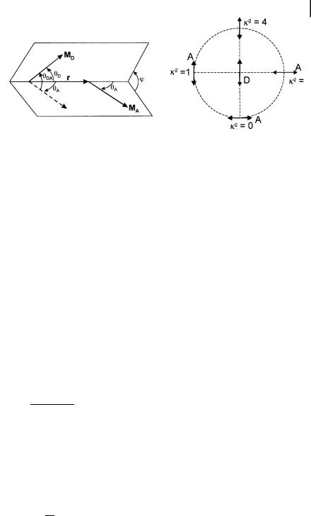
Fig. 4.17. Angles involved in the definition of the orientation factor k2 (left) and examples of values of k2 (right).

where yDA is the angle between the donor and acceptor transition moments, and yD and yA are the angles between these, respectively, and the separation vector; j is the angle between the projections of the transition moments on a plane perpendicular to the line through the centers (Fig. 4.17). k2 can in principle take values from 0 (perpendicular transition moments) to 4 (collinear transition moments). When the transition moments are parallel, k2 ¼ 1.

When the molecules are free to rotate at a rate that is much faster than the deexcitation rate of the donor (isotropic dynamic averaging), the average value of k2 is 2/3. In a rigid medium, the square of the average of k is 0.476 for an ensemble of acceptors that are statistically randomly distributed about the donor with respect to both distance and orientation (this case is often called the static isotropic average).

The transfer e ciency is defined as

Using Eq. (4.78), the transfer e ciency can be related to the ratio r=R0:

Note that the transfer e ciency is 50% when the donor–acceptor distance is equal to the Fo¨rster critical radius. Equation (4.83) shows that the distance between a donor and an acceptor can be determined by measuring the e ciency of transfer, provided that r is not too di erent from R0 (which is evaluated by means of Eq. 4.80).

The e ciency of transfer can also be written in the following form:

122 4 Effects of intermolecular photophysical processes on fluorescence emission

where tD0 and tD are the donor excited-state lifetimes in the absence and presence of acceptor, respectively.

The use of Fo¨rster non-radiative energy transfer for measuring distances at a supramolecular level (spectroscopic ruler) will be discussed in detail in Chapter 9.

Dexter’s formulation of exchange energy transfer (very weak coupling) In contrast to the inverse sixth power dependence on distance for the dipole–dipole mechanism, an exponential dependence is to be expected from the exchange mechanism. The rate constant for transfer can be written as

0y

where L is the average Bohr radius. Because K (Eq. 4.85) is a constant that is not related to any spectroscopic data, it is di cult to characterize the exchange mechanism experimentally.

Selection rules

1. Dipole–dipole mechanism:

.Equation (4.79) shows that R0, and consequently the transfer rate, is independent of the donor oscillator strength but depends on the acceptor oscillator strength and on the spectral overlap. Therefore, provided that the acceptor transition is allowed (spin conservation) and its absorption spectrum overlaps the donor fluorescence spectrum, the following types of energy transfer are possible:

1D þ 1A ! 1D þ 1A (singlet–singlet energy transfer) (e.g. anthracene þ perylene, or pyrene þ perylene).

1D þ 3A ! 1D þ 3A (higher triplet). This type of transfer requires overlap of the fluorescence spectrum of D and the TaT absorption spectrum of A (e.g. quenching of perylene by phenanthrene in its lowest triplet state).

3D þ 1A ! 1D þ 1A (triplet–singlet energy transfer). This type of transfer leads to phosphorescence quenching of the donor (e.g. phenanthrene (T) þ rhodamine B (S)).

13) Note that Ð0y IDðlÞeAðlÞ dl ¼ Ð0y IDðnÞeAðnÞ dn.

Bibliography

Andrews D. L. and Demidov A. A. (Eds)
(1999) Resonance Energy Transfer, Wiley, Chichester.
Berberan-Santos M. N., Pereira E. J. N. and Martinho J. M. G. (1999) Dynamics of Radiative Transport, in: Andrews D. L.
and Demidov A. A. (Eds), Resonance Energy Transfer, Wiley, Chichester, pp. 108– 150.
Birks J. B. (1970) Photophysics of Aromatic Molecules, Wiley, London.
Birks J. B. (Ed.) (1973) Organic Molecular Photophysics, Wiley, London.
Cheung H. C. (1991) Resonance Energy Transfer, in: Lakowicz J. R. (Ed.), Topics in Fluorescence Spectroscopy, Vol. 2, Principles, Plenum Press, New York, pp. 127–176.
Clegg R. M. (1996) Fluorescence Resonance Energy Transfer, in: Wang X. F. and Herman B. (Eds), Fluorescence Imaging Spectroscopy and Microscopy, Wiley, New York, pp. 179–252.
Dexter D. L. (1953) A Theory of Sensitized Luminescence in Solids, J. Chem. Phys. 21, 836–850.
Eftink M. R. (1991a) Fluorescence