Molecular Fluorescence

4.2 Overview of the intermolecular de-excitation processes of excited molecules 85

leads to

In contrast to the Stern–Volmer equation (4.10), the ratio I0=I is not linear and shows an upward curvature at high quencher concentrations. At low concentrations, expðVqNa½Q&ÞA1 þ VqNa½Q&, so that the concentration dependence is almost linear (as in the case of the Stern–Volmer plot).

A plot of lnðI0=IÞ versus [Q] yields Vq. The values of VqNa are often found to be in the range of 1–3 L mol 1. This corresponds to a quenching sphere radius of about 10 A˚ , which is somewhat larger than the van der Waals contact distance between M and Q.

Perrin’s model has been used in particular for the interpretation of non-radiative energy transfer in rigid media (see Chapter 9).

4.2.3.2 Formation of a ground-state non-fluorescent complex

Let us consider the formation of a non-fluorescent 1:1 complex according to the equilibrium

M þ Q SMQ

The excited-state lifetime of the uncomplexed fluorophore M is una ected, in contrast to dynamic quenching. The fluorescence intensity of the solution decreases upon addition of Q, but the fluorescence decay after pulse excitation is una ected. Quinones, hydroquinones, purines and pyrimidines are well-known examples of molecules responsible for static quenching.

Using the relation for the stability constant of the complex

Considering that the fluorescence intensities are proportional to the concentrations (which is valid only in dilute solutions), this relationship can be rewritten as

86 4 Effects of intermolecular photophysical processes on fluorescence emission

A linear relationship is thus obtained, as in the case of the Stern–Volmer plot (Eq. 4.10), but there is no change in excited-state lifetime for static quenching, whereas in the case of dynamic quenching the ratio I0=I is proportional to the ratio t0=t of the lifetimes.

In some cases, evidence for the formation of a complex can be obtained (e.g. changes in the absorption spectrum upon complexation), but in the absence of such evidence, the interaction is likely to be non-specific and the model of an effective sphere of quenching is more appropriate. A nonlinear variation of I0=I is predicted in the latter case, but at low quencher concentration, expðVqNa½Q&ÞA1 þ

VqNa½Q&.

The above considerations can be generalized to complexes of the type M Qn ðn > 1Þ. The probability that a molecule M is in contact with n quencher molecules can be approximately expressed by the Poisson distribution (Eq. 4.21). Perrin’s equation (4.23) is then found again.

An interesting application of static quenching is the determination of micellar aggregation numbers (see Box 4.2).

4.2.4

Simultaneous dynamic and static quenching

Static and dynamic quenching may occur simultaneously, resulting in a deviation of the plot of I0=I against [Q] from linearity.

Let us consider first the case of static quenching by formation of a nonfluorescent complex. The ratio I0=I obtained for dynamic quenching must be

An upward curvature is thus observed. KSV and KS can be determined by curve fitting using Eq. (4.29), or alternatively from the plot of ðI0=I 1Þ=½Q& against [Q], which should be linear.

Alternatively, using the sphere of e ective quenching model, we obtain the following relation instead of Eq. (4.29)

4.2 Overview of the intermolecular de-excitation processes of excited molecules 87

Box 4.2 Determination of micellar aggregation numbers by means of fluorescence quenchinga)

Method I: Static quenching by totally micellized quenchers

Let us consider a fluorescent probe and a quencher that are soluble only in the micellar pseudo-phase. If the quenching is static, fluorescence is observed only from micelles devoid of quenchers. Assuming a Poissonian distribution of the quencher molecules, the probability that a micelle contains no quencher is given by Eq. (4.22), so that the relationship between the fluorescence intensity and the mean occupancy number hni is

ln I0 ¼ hni ðB4:2:1Þ

I

hni is related to the micellar aggregation number Nag by the following relation:

where [Q] is the total concentration of quencher, [Mic] is the concentration of micelles, [Surf ] is the total concentration of surfactant and [CMC] is the critical micellar concentration. Nag can be calculated from this relation, when all the concentrations are known.

Static quenching by totally micellized quenchers provides a simple steadystate method for the determination of Nag. This method was originally employed with Ru(bpy)32þ as a fluorophore and 2-methylanthracene as a quencher in SDS (sodium dodecylsulfate) micelles. It is no longer applicable when the contribution of dynamic quenching is not negligible. The validity can be checked by time-resolved measurements: the fluorescence decay should indeed be a single exponential for pure static quenching. Otherwise, the relations given in Method II should be applied.

Method II: Dynamic quenching by totally micellized immobile quenchers

It is assumed that the probability of quenching of a fluorescent probe in a given micelle is proportional to the number of quenchers residing in this micelle. The rate constant for de-excitation of a probe in a micelle containing n quencher molecules is given by

where kq is the first-order rate constant for the quenching by one quencher molecule (the intramicellar quenching process is assumed to be a first-order process, as for intramolecular processes).

4.2 Overview of the intermolecular de-excitation processes of excited molecules 89

In a logarithmic representation, the slope at long times is the same as in the absence of quencher, and extrapolation to time 0 yields hni, from which Nag can be calculated as in Method I.

Quenching of pyrene by excimer formation (Py þ Py ! (PyPy) ! 2Py) (see Section 4.4.1) is widely used for the determination of micellar aggregation numbers for new surfactant systems. An example is given in Figure B4.2.1.

Fluorescence quenching studies in micellar systems provide quantitative information not only on the aggregation number but also on counterion binding and on the e ect of additives on the micellization process. The solubilizing process (partition coe cients between the aqueous phase and the micellar pseudo-phase, entry and exit rates of solutes) can also be characterized by fluorescence quenching.

For example, this relation has been successfully used to describe oxygen quenching of perylene in dodecane at high oxygen pressure.

It should be recalled that an upward curvature can also be due to transient e ects that may superimpose the e ects of static quenching. The following general relation can then be used

where Y is given by Eq. (4.19).

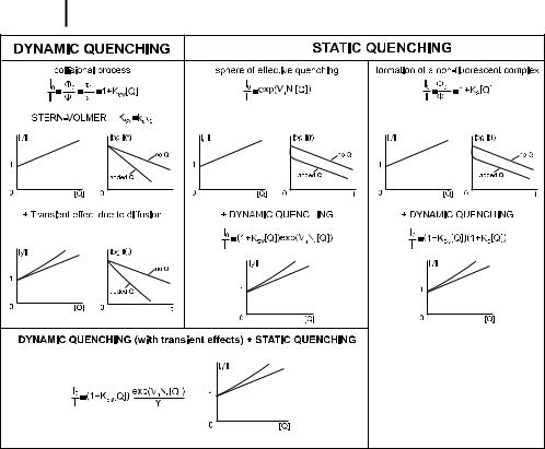
Figure 4.2 summarizes the various cases of quenching, together with the possible origins of a departure from a linear Stern–Volmer plot.

It should be emphasized that time-resolved experiments are required for unambiguous assignment of the dynamic and static quenching constants.

4.2.5

Quenching of heterogeneously emitting systems

When a system contains a fluorophore in di erent environments (e.g. a fluorophore embedded in microheterogeneous materials such as sol–gel matrices, polymers, etc.) or more than one fluorophore (e.g. di erent tryptophanyl residues of a protein), the preceding relations must be modified. If dynamic quenching is predominant, the Stern–Volmer relation should be rewritten as

90 4 Effects of intermolecular photophysical processes on fluorescence emission

Fig. 4.2. Distinction between dynamic and static quenching.

where KSV; i is the Stern–Volmer constant for the ith species and fi is the fractional contribution of the ith species to the total fluorescence intensity for a given couple of selected excitation and observation wavelengths. If the values of KSV; i and fi are quite di erent, a downward curvature of I0=I is observed.

In the case of additional static quenching, Eq. (4.32) becomes

4.3

Photoinduced electron transfer

Photoinduced electron transfer (PET) is often responsible for fluorescence quenching. This process is involved in many organic photochemical reactions. It plays a major role in photosynthesis and in artificial systems for the conversion of solar energy based on photoinduced charge separation. Fluorescence quenching experiments provide a useful insight into the electron transfer processes occurring in these systems.

4.3 Photoinduced electron transfer 91

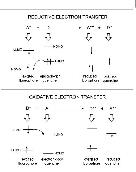
Fig. 4.3. Reductive and oxidative electron transfers.

The oxidative and reductive properties of molecules can be enhanced in the excited state. Oxidative and reductive electron transfer processes according to the following reactions:

1D þ A ! Dþ þ A

1A þ D ! A þ Dþ

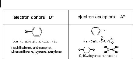
are schematically illustrated in Figure 4.3. Examples of donor and acceptor molecules are given in Figure 4.4.

92 4 Effects of intermolecular photophysical processes on fluorescence emission

Fig. 4.4. Examples of electron donors and acceptors in the excited state.

In the gas phase, the variations in standard free enthalpy DG0 for the above reactions can be expressed using the redox potentials E0 and the excitation energy DE00, i.e. the di erence in energy between the lowest vibrational levels of the excited state and the ground state:

These equations are called Rehm–Weller equations. If the redox potentials are expressed in volts, DG0 is then given in volts. Conversion into J mol 1 requires multiplication by the Faraday constant (F ¼ 96 500 C mol 1).

In solution, two terms need to be added to take into account the solvation e ect (enthalpic term DHsolv) and the Coulombic energy of the formed ion pair:

where e is the electron charge, e is the dielectric constant of the solvent and r is the distance between the two ions.

The redox potentials can be determined by electrochemical measurements or by theoretical calculations using the energy levels of the LUMO (lowest unoccupied molecular orbital) and the HOMO (highest occupied molecular orbital).

In solution, electron transfer reactions can be described by Schemes 4.2 or 4.3. If the reaction is not di usion-limited, the reaction rate kR, denoted here kET for electron transfer, can be determined. Two cases are possible.

.If the interaction between the donor and acceptor in the encounter pair is strong (Scheme 4.3), this encounter pair (DA) is called an ‘exciplex’ (see Section 4.4).

4.3 Photoinduced electron transfer 93

.If the interaction between the donor and acceptor in the encounter pair (D . . .A) is weak (Scheme 4.2), the rate constant kET can be estimated by the Marcus theory. This theory predicts a quadratic dependence of the activation free energy DG versus DG0 (standard free energy of the reaction).

where lin is the contribution due to changes in the intramolecular bond length and bond angle in the donor and acceptor during electron transfer, and ls is the contribution of the solvent reorganization.

In the framework of the collision theory, kET can then be evaluated by means of the usual relation

where Z is the frequency of collisions and DG is the free energy of activation for the ET process.

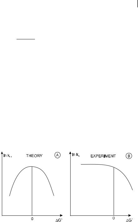
Because of the quadratic dependence, the variation of lnðkETÞ versus DG0 is expected to be a parabol whose maximum corresponds to DG0 ¼ 0 (Figure 4.5). Beyond the maximum ðDG0 > 0Þ, kET decreases when DG0 increases (normal region), whereas below the maximum ðDG0 < 0Þ, the inverse behavior is expected (Marcus’ inverse region).

Fig. 4.5. Variations of the rate constant for electron transfer versus DG0 according to the Marcus theory.

94 4 Effects of intermolecular photophysical processes on fluorescence emission

The theoretical prediction has been confirmed in the normal region by fluorescence quenching experiments in which the observed rate constant kq is directly representative of the rate constant kET for electron transfer. Conversely, the inverse region has not been observed for intermolecular ET because in the inverse region, where DG0 f0, kET is so large (according to Eqs 4.40 and 4.38) that the reaction is di usion-limited (kR ¼ kET gk1 in Scheme 4.2); in other words, kq ¼ k1 so that the Marcus theory is irrelevant. Consequently, when DG0 becomes more and more negative, kq reaches a plateau corresponding to the di usional rate constant k1 (Figure 4.5B), whereas a decrease is predicted by the Marcus theory.

Nevertheless, the inverse region is observed in the particular case where the electron donor and the electron acceptor are held apart by a bridge (e.g. porphyrins covalently linked to quinones).

4.4

Formation of excimers and exciplexes

Excimers are dimers in the excited state (the term excimer results from the contraction of ‘excited dimer’). They are formed by collision between an excited molecule and an identical unexcited molecule:

1M þ 1M T 1ðMMÞ

The symbolic representation (MM) shows that the excitation energy is delocalized over the two moieties (as in an excitonic interaction described in Section 4.6).

Exciplexes are excited-state complexes (the term exciplex comes from ‘excited complex’). They are formed by collision of an excited molecule (electron donor or acceptor) with an unlike unexcited molecule (electron acceptor or donor):

1D þ A T 1ðDAÞ

1A þ D T 1ðDAÞ

The formation of excimers and exciplexes are di usion-controlled processes. The photophysical e ects are thus detected at relatively high concentrations of the species so that a su cient number of collisions can occur during the excited-state lifetime. Temperature and viscosity are of course important parameters.

4.4.1

Excimers

Many aromatic hydrocarbons such as naphthalene or pyrene can form excimers. The fluorescence band corresponding to an excimer is located at wavelengths higher than that of the monomer and does not show vibronic bands (see Figure 4.6 and the example of pyrene in Figure 4.7).