

Molecular Fluorescence
.pdf5.6 Effect of rotational Brownian motion 145
The e ect of Brownian rotation is thus simply expressed by multiplying the second
member of Eq. (5.27) by ð3 cos2 oðtÞ 1Þ=2:
|
|
|
|
|
|
|
|
|
|
|
|
|
|
|
|
|
|
|
|
|
r t |
3 cos2 yEðtÞ 1 |
3 cos2 |
yAð0Þ 1 |
|
3 cos2 a 1 |
|
3 cos2 oðtÞ 1 |
|
5:31 |
|||||||||||
¼ |
|
|
|
|
ð |
|||||||||||||||
ð Þ¼ |
|
|
2 |
|
|
|
2 |
|
2 |
|
2 |
|
Þ |
|||||||
|
|
|
|
|
|
|
|
|
|
|
|
|
|
|
|
|
|
|
|
|
|
|
|
|
|
|
|
|
|
|
|
|
|
|
|
|
|
|
|
||
r t |
|
r |
3 cos2 oðtÞ 1 |
|
|
|
|
|
|
|
|
|
|
|
ð |
5:32 |
||||
ð Þ ¼ |
0 |
2 |
|
|
|
|
|
|
|
|
|
|
|
|
|
Þ |
||||
The quantity ð3 cos2 oðtÞ 1Þ=2 is the orientation autocorrelation function: it represents the probability that a molecule having a certain orientation at time zero is oriented at o with respect to its initial orientation. The quantity ð3x 1Þ=2 is the Legendre polynomial of order 2, P2ðxÞ, and Eq. (5.32) is sometimes written in the following form
rðtÞ ¼ r0hP2½cos oðtÞ&i |
ð5:33Þ |
The angled brackets hi indicate an average over all excited molecules8).
Isotropic rotations
Let us consider first the case of spherical molecules. Their rotations are isotropic and the average of cos2 oðtÞ can be calculated by the integral:
y |
|
|
cos2 oðtÞ ¼ ð0 |
cos2 oWðo; tÞ sin o do |
ð5:34Þ |
where Wðo; tÞ represents the orientation distribution function expressing the probability that a molecule has an orientation o at time t, taking into account that o ¼ 0 at time zero. This function must fulfill the following conditions and equations:
. |
initial condition: Wð0; 0Þ ¼ 1 |
|
. |
normalization condition |
|
|
ðp |
ð5:35Þ |
|
2p Wðo; tÞ sin o do ¼ 1 |
0
8)It is interesting to note that in dielectric relaxation experiments, the orientation autocorrelation function that is involved in the theory is
hP1½cos oðtÞ&i ¼ cos oðtÞ

146 5 Fluorescence polarization. Emission anisotropy
. Brownian di usion equation for a spherical particle
qWðo; tÞ |
¼ |
D |
‘2W o; t |
ð |
5:36 |
|
qt |
||||||
r |
ð Þ |
Þ |
where Dr is the rotation di usion coe cient. In spherical coordinates, Eq. (5.36) can be rewritten as
qW |
|
|
1 q |
qW |
|
|
|||||||
|
|
|
¼ Dr |
|
|
|
|
|
sin o |
|
|
ð5:37Þ |
|
|
qt |
sin o |
qo |
qo |
|||||||||
|
|
|
|
|
|||||||||
By setting cos2 oðtÞ ¼ u, the above equations lead to |
|
||||||||||||
du |
|
|
|
|
|
|
|
|
|
|
|
||
|
|
¼ 2Dr 6Dru |
|
|
|
ð5:38Þ |
|||||||
|
dt |
|
|
|
|||||||||
Taking into account the initial condition cos2 oð0Þ ¼ 1, the solution of this equation is
1 |
½1 þ 2 expð 6DrtÞ& |
|
|||
|
u ¼ |
|
ð5:39Þ |
||
|
3 |
||||
The autocorrelation function ð3u 1Þ=2 is then a single exponential |
|
||||
|
hP2½cos oðtÞ&i ¼ expð 6DrtÞ |
ð5:40Þ |
|||
Hence |
|
||||
|
|
|
|
|
|
|
rðtÞ ¼ r0 expð 6DrtÞ |
|
ð5:41Þ |
||
Dr can be determined by time-resolved fluorescence polarization measurements, either by pulse fluorometry from the recorded decays of the polarized components Ik and I?, or by phase fluorometry from the variations in the phase shift between Ik and I? as a function of frequency (see Chapter 6). If the excited-state lifetime is unique and determined separately, steady-state anisotropy measurements allow us to determine Dr from the following equation, which results from Eqs (5.10) and (5.41):
1 |
1 |
ð1 þ 6DrtÞ |
ð5:42Þ |
||||
|
|
|
|
¼ |
|
||
|
|
|
|
r0 |
|||
|
r |
||||||
|
|
|
|
|
|
|
|
This relationship is called Perrin’s equation, because it was established for the first time by Francis Perrin; it was written at that time with polarization ratios
1 |
|
1 |
1 |
|
1 |
|
||||
|
|
|
|
|
¼ |
|
|
|
ð1 |
þ 6DrtÞ |
p |
3 |
p0 |
3 |
|||||||

5.6 Effect of rotational Brownian motion 147
Once Dr is determined by fluorescence polarization measurements, the Stokes– Einstein relation can be used:
Dr ¼ |
RT |
ð5:43Þ |
6Vh |
where V is the hydrodynamic molecular volume of the fluorophore, h is the viscosity of the medium, T is the absolute temperature and R is the gas constant. However, it should be emphasized that the validity of the Stokes–Einstein relation is questionable on a molecular scale (see Chapter 8). In particular, it is not valid to assign a numerical value to the viscosity of a microenvironment from fluorescence polarization measurements in conjunction with the Stokes–Einstein relation.
Equations (5.41) and (5.42) are often written with the rotational correlation time tc ¼ 1=ð6DrÞ
rðtÞ ¼ r0 expð t=tcÞ |
ð5:44Þ |
||||||||
1 |
1 |
1 |
|
t |
|
|
|||
|
|
|
¼ |
|
þ |
|
ð5:45Þ |
||
|
|
|
r0 |
tc |
|||||
r |
|||||||||
We have considered spherical molecules so far, but it should be noted that isotropic rotations can also be observed in the case of molecules with cylindrical symmetry and whose absorption and emission transition moments are parallel and oriented along the symmetry axis. In fact, any rotation around this axis has no e ect on the fluorescence polarization. Only rotations perpendicular to this axis have an e ect. A typical example is diphenylhexatriene whose transition moment is very close to the molecular axis (see Chapter 8).
Anisotropic rotations
In most cases, fluorescent molecules undergo anisotropic rotations because of their asymmetry. A totally asymmetric rotor has three di erent rotational di usion coe cients, and in cases where the absorption and emission transition moments are not directed along one of the principal di usion axes, the decay of rðtÞ is a sum of five exponentials (see Box 5.3).
When the instantaneous emission anisotropy rðtÞ is a sum of exponentials
rðtÞ ¼ r0 |
Xi |
ai expð t=tciÞ |
ð5:46Þ |
|||||
the steady-state anisotropy is given by |
|
|||||||
|
|
¼ r0 Xi |
|
|
ai |
|
ð5:47Þ |
|
r |
|
|
||||||
|
1 |
|
t=tci |
|||||
|
|
|
|
|
þ |
|
||
Steady-state anisotropy measurements are then insu cient for fully characterizing rotational motions and time-resolved experiments are required.

148 5 Fluorescence polarization. Emission anisotropy
Box 5.3 Emission anisotropy of totally asymmetric rotors and ellipsoids
A totally asymmetric rotor has three di erent rotational di usion coe cients D1, D2 and D3, around the three principal di usion axes of the molecule (which are di erent from the laboratory axes x, y and z). In cases where the absorption and emission transition moments are not directed along one of the principal axes, the decay of rðtÞ is a sum of five exponential terms. There was originally some controversy about the expression of rðtÞa–d). The correct solution was derived by Belford et al.d)
6 X3
rðtÞ ¼ 5 i¼1 Ci expð t=tiÞ þ ½ðF þ GÞ=4& expð 6D 2DÞt
þ ½ðF GÞ=4& expð 6D þ 2DÞt
where D, the mean rotational di usion coe cient, D, Ci and F are given by
D ¼ ðD1 þ D2 þ D3Þ=3
D ¼ ðD12 þ D22 þ D32 D1D2 D1D3 D2D3Þ1=2
Ci ¼ ajakejek ði; j; k ¼ 123; 231 or 321Þ
where a1, a2 and a3 are the cosines of the angles formed by the absorption transition moments with the three principal axes, and e1, e2 and e3 are the corresponding direction cosines of the emission transition moments.
ti ¼ 1=ð3D þ 3DiÞ
X3
F ¼ ai2ei2 1=3
i¼1
X3
GD ¼ Diðai2ei2 þ aj2ek2 þ ak2ej2Þ D i 0j 0k i¼1
For a particle with spherical symmetry ðD1 ¼ D2 ¼ D3 ¼ DÞ, the above expression reduces to Eq. (5.41).
In the particular case of prolate and oblate ellipsoids, the number of exponentials is reduced to three because two of the three axes are equivalent. The rotation di usion coe cients around the axis of symmetry and the equatorial axis are denoted D1 and D2, respectively. The emission anisotropy can then be written as
rðtÞ ¼ a1 exp½ 6D2t& þ a2 exp½ ðD1 þ 5D2Þt& þ a3 exp½ ð4D1 þ 2D2Þt&

5.6 Effect of rotational Brownian motion 149
where the pre-exponential factors depend on the orientation of the transition moments with respect to the ellipsoid axes as follows:
a1 ¼ 0:1ð3 cos2 y1 1Þð3 cos2 y2 1Þ
a2 ¼ 0:3 sin 2y1 sin 2y2 cos f
a3 ¼ 0:3 sin2 y1 sin2 y2ðcos2 f sin2 fÞ
where y1 and y2 are the angles formed by the absorption and emission transitions moments, respectively, with the axis of symmetry of the ellipsoid, and f is the angle formed by the projections of the two moments in the plane perpendicular to the axis of symmetry.
When the absorption and emission transition moments are collinear (y1 ¼ y2 ¼ y and f ¼ 0), the pre-exponential factors become
a1 ¼ 0:1ð3 cos2 y 1Þ2
a2 ¼ 0:3 sin2 2y
a3 ¼ 0:3 sin4 y
In the case of an ellipsoid of revolution for which the absorption or emission transition moment is parallel to the axis of symmetry (y1 or y2 ¼ 0), the anisotropy decay is a single exponential
rðtÞ ¼ 0:4 expð 6D2tÞ
A more complex expression is obtained when the absorption and emission transition moments lie in a plane perpendicular to the axis of symmetry
rðtÞ ¼ 0:1 expð 6D2tÞ þ 0:3ð2 cos2 a 1Þ exp½ ð4D1 þ 2D2Þt&
where a is the angle between the absorption and emission transition moments. In the particular case where this angle is 45 , this expression reduces to the first term.
In principle, the shape parameters of asymmetric rotors can be estimated from time-resolved anisotropy decay measurements, but in practice it is di cult to obtain accurate anisotropy decay curves over much more than one decade, which is often insu cient to determine more than two rotational correlation times.
a) Tao T. (1969) Biopolymers 8, 609. |
Phys. Lett. 14, 539. |
b) Chuang, T. J. and Eisenthal K. B. (1972) J. |
d) Belford G. G., Belford R. L. and Weber G. |
Chem. Phys. 57, 5094. |
(1972) Proc. Natl. Acad. Sci. USA, 69, 1392. |
c) Ehrenberg M. and Rigler R. (1972) Chem. |
|
1505 Fluorescence polarization. Emission anisotropy
5.6.2
Hindered rotations
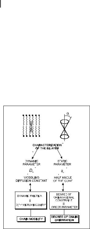
Special attention should be paid to anisotropic media such as lipid bilayers and liquid crystals. Let us consider first the ‘wobble-in-cone’ model (Kinosita et al., 1977; Lipari and Szabo, 1980) in which the rotations of a rod-like probe (with the direction of its absorption and emission transition moments coinciding with the long molecular axis) are restricted within a cone. The rotational motions are described by the rotational di usion coe cient Dw around an axis perpendicular to the long molecular axis (the rotations around this axis having no e ect on the emission anisotropy) and an order parameter (half-angle of the cone yc) reflecting the degree of orientational constraint due to the surrounding para nic chains (Figure 5.12). yc can be determined from the ratio r=r0:
ry |
1 |
|
|
|
|
2 |
|
|
|
||
|
|
|
|
|
|
|
|
||||
|
¼ |
|
|
cos ycð1 þ cos ycÞ |
ð5:48Þ |
||||||
r0 |
2 |
||||||||||
|
|
|
|
|
|
|
|
|
|
|
|
|
|
|
|
|
|
|
|
|
|
|
|
|
|
|
|
|
|
|
|
|
|
|
|
|
|
|
|
|
|
|
|
|
|
|
|
Fig. 5.12. ‘Wobble-in-cone’ model for the characterization of bilayers. The absorption and emission moments are assumed to coincide with the long molecular axis.

5.7 Applications 151
An approximate expression of the anisotropy decay is
rðtÞ ¼ ðr0 ryÞ expð t=tcÞ þ ry |
ð5:49Þ |
where tc is the e ective relaxation time of rðtÞ, i.e. the time in which the initially photoselected distribution of orientations approaches the stationary distribution. This time is related to Dw and yc by:
tcDw 1 |
ry |
|
2 |
|
2 |
|
|
|
¼ x0 |
ð1 |
þ x0Þ |
fln½ð1 þ x0Þ=2& þ ð1 þ x0Þ=2g=½2ð1 |
þ x0Þ& |
||
r0 |
|||||||
|
|
|
þ ð1 þ x0Þð6 þ 8x0 x02 12x03 7x04Þ=24 |
ð5:50Þ |
|||
where x0 ¼ cos yc.
In practice, the parameters r0, ry and tc are obtained from the best fit of IkðtÞ and I?ðtÞ given by Eqs (5.7) and (5.8), in which rðtÞ has the form of Eq. (5.49). Then, yc is evaluated from ry=r0, and Eq. (5.50) allows us to calculate the wobbling di usion constant Dw.
If data analysis with a single exponential decay is not satisfactory, a double exponential can be used, but such a decay must be considered as a purely mathematical model.
It is interesting to note that tcð1 ry=r0Þ is exactly the area A under ½rðtÞ ry&=r0. Therefore, even if the anisotropy decay is not a single exponential, Dw can be determined by means of Eq. (5.50) in which tcð1 ry=r0Þ is replaced by the measured area A. An example of application of the wobble-in-cone model to the study of vesicles and membranes is given in Chapter 8 (Box 8.3). More general theories have also been developed (see Box 5.4).
5.7
Applications
The various fields concerned with the applications of fluorescence polarization are listed in Table 5.1.
The fluorescence polarization technique is a very powerful tool for studying the fluidity and orientational order of organized assemblies (see Chapter 8): aqueous micelles, reverse micelles and microemulsions, lipid bilayers, synthetic non-ionic vesicles, liquid crystals. This technique is also very useful for probing the segmental mobility of polymers and antibody molecules. Information on the orientation of chains in solid polymers can also be obtained.
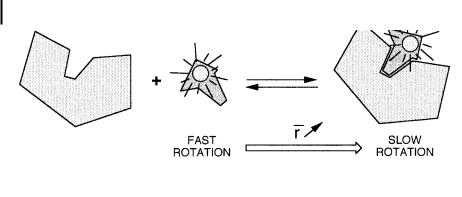
Fluorescence polarization is also well suited to equilibrium binding studies when the free and bound species involved in the equilibrium have di erent rotational rates (Scheme 5.1). Most molecular interactions can be analyzed by this method. It should be emphasized that, in contrast to other methods using tracers, fluorescence polarization provides a direct measurement of the ratio of bound and free tracer without prior physical separation of these species. Moreover, measure-

152 5 Fluorescence polarization. Emission anisotropy
Box 5.4 General model for hindered rotationsa–f )
The wobble-in-cone model has been generalized by introducing three autocorrelation functions G0ðtÞ, G1ðtÞ and G2ðtÞ into the expression for rðtÞ
rðtÞ ¼ r0½G0ðtÞ þ 2G1ðtÞ þ 2G2ðtÞ&
The values of these autocorrelation functions at times t ¼ 0 and t ¼ y are related to the two order parameters hP2i and hP4i, which are orientational averages of the secondand fourth-rank Legendre polynomial P2ðcos bÞ and P4ðcos bÞ, respectively, relative to the orientation b of the probe axis with respect to the normal to the local bilayer surface or with respect to the liquid crystal direction. The order parameters are defined as
hP2i ¼ h3 cos2 b 1i=2
hP4i ¼ h35 cos4 b 30 cos2 b þ 3i=8
and the autocorrelation functions are given by
G0ðtÞ ¼ |
1 |
|
þ |
2 |
hP2i |
þ |
18 |
hP4i |
||||||
|
|
|
|
|
|
|||||||||
5 |
7 |
35 |
||||||||||||
G1ðtÞ ¼ |
1 |
|
þ |
1 |
hP2i |
|
12 |
hP4i |
||||||
|
|
|
|
|
|
|||||||||
5 |
7 |
35 |
||||||||||||
G2ðtÞ ¼ 4 |
1 |
|
|
|
2 |
|
3 |
|
||||||
|
|
|
|
|
hP2i þ |
|
hP4i |
|||||||
5 |
7 |
35 |
||||||||||||
G0ðyÞ ¼ hP2i2
G1ðyÞ ¼ G2ðyÞ ¼ 0
It is assumed that the probe molecules undergo Brownian rotational motions with an angle-dependent ordering potential UðbÞ
UðbÞ ¼ kT½l2P2ðcos bÞ þ l4P4ðcos bÞ&
For a rod-like probe with its absorption transition moment direction coinciding with the long molecular axis, the rotational motion in this potential well is described by the di usion coe cient D?. The decay of the autocorrelation functions is then shown to be an infinite sum of exponential terms:
Xy
GkðtÞ ¼ bkm expð akmD?tÞ k ¼ 0; 1; 2
m¼0

5.7 Applications 153
The coe cients akm and bkm are complex functions of the parameters l2 and l4 that describe the ordering potential. In many practical situations, GkðtÞ is essentially mono-exponential:
GkðtÞ ¼ ½Gkð0Þ GkðyÞ& expð ak1D?tÞ þ GkðyÞ
The di usion constant D? with the underlying ‘microviscosity’, and the two order parameters hP2i, hP4i reflecting the degree of orientational constraint have been successfully determined from the fluorescence anisotropy decay in vesicles and liquid crystals.
a) Van der Meer W., Kooyman R. P. H. and |
d) Szabo A. (1984) J. Chem. Phys. 81, 150. |
Levine Y. K. (1982) Chem. Phys. 66, 39. |
e) Fisz J. J. (1985) Chem. Phys. 99, 177; ibid. |
b) Van der Meer W., Pottel H., Herreman W., |
(1989) 132, 303; ibid. (1989) 132, 315. |
Ameloot M., Hendrickx H. and Schro¨der H. |
f ) Pottel H., Herreman W., Van der Meer B. |
(1984) Biophys. J., 46, 515. |
W. and Ameloot M. (1986) Chem. Phys. 102, |
c) Zannoni C., Arcioni A. and Cavatorta P. |
37. |
(1983) Chem. Phys. Lipids 32, 179. |
|
|
|
ments are carried out in real time, thus giving information on the kinetics of association and dissociation reactions.
Immunoassays based on fluorescence polarization have become very popular because, in contrast to radioimmunoassays, they require no steps to separate free and bound tracer. In a fluoroimmunoassay, the fluorescently labeled antigen is
Tab. 5.1. Fields of application of fluorescence polarization
Field |
Information |
|
|
Spectroscopy |
Excitation polarization spectra: distinction between excited |
|
states |
Polymers |
Chain dynamics |
|
Local viscosity in polymer environments |
|
Molecular orientation in solid polymers |
|
Migration of excitation energy along polymer chains |
Micellar systems |
Internal ‘microviscosity’ of micelles |
|
Fluidity and order parameters (e.g. bilayers of vesicles) |
Biological membranes |
Fluidity and order parameters |
|
Determination of the phase transition temperature |
|
E ect of additives (e.g. cholesterol) |
Molecular biology |
Proteins (size, denaturation, protein–protein interactions, |
|
etc.) |
|
DNA–protein interactions |
|
Nucleic acids (flexibility) |
Immunology |
Antigen–antibody reactions |
|
Immunoassays |
Artificial and natural antennae |
Migration of excitation energy |
|
|
154 5 Fluorescence polarization. Emission anisotropy
Scheme 5.1
bound to an antibody such that most of the antigen is bound, thereby maximizing the value of emission anisotropy. Upon addition of unlabeled antigen, bound labeled antigen will be displaced from the antibody and the emission anisotropy will decrease accordingly.
Finally, energy migration, i.e. excitation energy hopping, in polymers, artificial antenna systems, photosynthetic units, etc. can be investigated by fluorescence polarization (see Chapter 9).
5.8
Bibliography
Kinosita K., Kawato S. and Ikegami A.
(1977) A Theory of Fluorescence Polarization Decay in Membranes, Biophys. J. 20, 289–305.
Lipari G. and Szabo A. (1980) E ect of Vibrational Motion on Fluorescence Depolarization and Nuclear Magnetic Resonance Relaxation in Macromolecules and Membranes, Biophys. J. 30, 489–506.
Steiner R. F. (1991) Fluorescence Anisotropy: Theory and Applications, in: Lakowicz J. R. (Ed.), Topics in Fluorescence Spectroscopy, Vol. 2, Principles, Plenum Press, New York, pp.
127–176.
Thulstrup E. W. and Michl J. (1989)
Elementary Polarization Spectroscopy, VCH, New York.
Valeur B. (1993) Fluorescent Probes for Evaluation of Local Physical, Structural Parameters, in: Schulman S. G. (Ed.),
Molecular Luminescence Spectroscopy. Methods and Applications, Part 3, Wiley-Interscience, New York, pp. 25–84.
Weber G. (1953) Rotational Brownian Motions and Polarization of the Fluorescence of Solutions, Adv. Protein Chem. 8, 415–459.