

Molecular Fluorescence
.pdf
346 10 Fluorescent molecular sensors of ions and molecules
Tab. 10.B.1. Relative values of the stability constants in the case of n identical and independent binding sites (Connors, 1987)
n |
K11 |
K21 |
K31 |
K41 |
K51 |
K61 |
2 |
2 |
1=2 |
|
|
|
|
3 |
3 |
1 |
1=3 |
|
|
|
4 |
4 |
3=2 |
2=3 |
1=4 |
|
|
5 |
5 |
2 |
1 |
1=2 |
1=5 |
|
6 |
6 |
5=2 |
4=3 |
3=4 |
2=5 |
1=6 |
|
|
|
|
|
|
|
.negatively cooperative (or anti-cooperative) if the ratio Kðiþ1Þ1=Ki1 is smaller than the statistical value.
In particular, for a ditopic receptor that can bind successively two cations (see previous section), the criterion for cooperativity is K21=K11 > 1=4, i.e. complexation of a second cation is made easier by the presence of a bound cation. For instance, a cooperative e ect was observed with fluoroionophore E-1 (see Section 10.3.4).
Determination of the stoichiometry of a complex by the method of continuous variations ( Job’s method)
An assumed 1:1 stoichiometry for a complex can be confirmed or invalidated by the fit of the titration curves described above for this case. If the fit is not satisfactory, a model of formation of two successive complexes can be tried.
Information on the stoichiometry of a complex can also be obtained from the continuous variation method (see Connors, 1987). Let us consider a complex MmLl formed according to the equilibrium
mM þ lL Ð MmLl
with |
|
|
|
||
b |
ml ¼ |
½MmLl& |
ð |
B:31 |
|
½M&m½L&l |
|||||
|
Þ |
||||
The principle of the method as follows: the absorbance or the fluorescence intensity Y is measured for a series of solutions containing the ligand and the cation such that the sum of the total concentrations of ligand and cation is constant.
cL þ cM ¼ C ¼ constant |
ðB:32Þ |
The position of the maximum of Y is then related to the ratio m=l, as shown below. It is convenient to use the following dimensionless quantity (which is analogous
to a molar fraction but not strictly):

|
|
|
|
10.6 Towards fluorescence-based chemical sensing devices |
347 |
||
x ¼ |
cM |
cM |
|
|
|||
ðB:33Þ |
|||||||
|
¼ |
|
|
||||
cM þ cL |
C |
||||||
Mass balance equations are |
|
|
|||||
cL ¼ ½L& þ l½MmLl& |
ðB:34Þ |
||||||
cM ¼ ½M& þ m½MmLl& |
ðB:35Þ |
||||||
These equations can be rewritten as |
|
|
|||||
Cð1 xÞ ¼ ½L& þ l½MmLl& |
ðB:36Þ |
||||||
Cx ¼ ½M& þ m½MmLl& |
ðB:37Þ |
||||||
Combination of Eqs (B.31)–(B.37) gives |
|
|
|||||
bmlfCx m½MmLl&gmfCð1 xÞ l½MmLl&gn ¼ ½MmLl& |
ðB:38Þ |
||||||
Taking the logarithm of this expression, then di erentiating with respect to x, and finally setting d½MmLl&=dx ¼ 0, we obtain
|
m |
¼ |
xmax |
|
ðB:39Þ |
|
l |
1 xmax |
|||
This treatment assumes that a single complex is present, but this assumption may not be valid. When only one complex is present, the value of xmax is independent of the wavelength at which the absorbance or fluorescence intensity is measured. A dependence on wavelength is an indication of the presence of more than one complex.
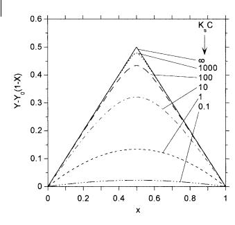
For a 1:1 complex, xmax ¼ 12 , according to Eq. (B.39). To illustrate the shape of Job’s plot, the following equation can be derived with the same notations as above:
Y |
|
aC |
1 |
|
x |
|
ðb aÞC |
81 |
|
1 |
" |
1 |
|
1 2 |
4x |
1 |
|
x |
Þ# |
1=2 |
9 |
B:40 |
|
|
|
|
|
|
|
|
|
|
|
||||||||||||||
¼ |
|
Þ þ |
2 |
þ KsC |
þ KsC |
|
|
||||||||||||||||
|
ð |
|
|
< |
|
ð |
|
|
|
= |
ð Þ |
||||||||||||
|
|
|
|
|
|
|
|
: |
|
|
|
|
|
|
|
|
|
|
|
|
|
; |
|
where a and b have the same meaning as in Eqs (B.8) and (B.9). The product aC is equal to Y0, i.e. the value of Y when no cation is added ðx ¼ 0Þ.
When plotting the variations in absorbance or fluorescence intensity versus x, it is convenient to subtract the absorbance or fluorescence intensity that would be measured in the absence of cation at every concentration, i.e. Y0ð1 xÞ. In this way, the plot of Y Y0ð1 xÞ versus x starts from 0 for x ¼ 0, goes through a maximum, and returns to 0 for x ¼ 1. Equation (B.40) can thus be rewritten as
Y |
|
Y0 |
|
1 |
|
x |
|
ðb=a 1ÞY0 |
81 |
|
1 |
" |
1 |
|
1 2 |
4x 1 |
x |
Þ# |
1=2 |
9 |
B:41 |
|
|
|
|
|
|
|
|
|
|
|
|||||||||||||
|
ð |
|
Þ ¼ |
2 |
þ KsC |
þ KsC |
|
|||||||||||||||
|
|
|
|
< |
|
ð |
|
|
= |
ð Þ |
||||||||||||
|
|
|
|
|
|
|
|
|
: |
|
|
|
|
|
|
|
|
|
|
|
; |
|
|
10.7 Bibliography |
349 |
Czarnik A. W. (Ed.) (1993) Fluorescent |
|
|
Hartmann W. K., Mortellaro M. A., Nocera |
||
Chemosensors for Ion and Molecule |
D. G. and Pikramenou Z. (1997) |
|
Recognition, ACS Symposium Series 358, |
Chemosensing of Monocyclic and Bicyclic |
|
American Chemical Society, Washington, |
Aromatic Hydrocarbons by Supramolecular |
|
DC. |
Active Sites, in: Desvergne J.-P. and |
|
Czarnik A. W. (1994) Chemical |
Czarnik A. W. (Eds), Chemosensors of Ion |
|
Communication in Water Using |
and Molecule Recognition, NATO ASI series, |
|
Fluorescent Chemosensors, Acc. Chem. Res. |
Kluwer Academic Publishers, Dordrecht, |
|
27, 302–8. |
pp. 159–76. |
|
de Silva A. P., Gunaratne H. Q. N., |
Haugland R. P., Handbook of Fluorescent |
|
Gunnlaugsson T., Huxley A. J. M., |
Probes and Research Chemicals, 6th edn, |
|
McCoy C. P., Rademacher J. T. and Rice T. |
Molecular Probes, Inc., Eugene, OR, |
|
E. (1997) Signaling Recognition Events with |
USA. |
|
Fluorescent Sensors and Switches, Chem. |
Janata J. (1992) Ion Optodes, Anal. Chem. 64, |
|
Rev. 97, 1515–66. |
A921–7. |
|
Desvergne J.-P. and Czarnik A. W. (Eds) |
Jayaraman S., Biwersi J. and Verkman A. S. |
|
(1997) Chemosensors of Ion and Molecule |
(1999) Synthesis and Characterization of |
|
Recognition, NATO ASI series, Kluwer |
Dual-Wavelength Cl -Sensitive Fluorescent |
|
Academic Publishers, Dordrecht. |
Indicators for Ratio Imaging, Am. J. Physiol. |
|
Fabbrizzi L. and Poggi A. (1995) Sensors |
276, C747–57. |
|
and Switches from Supramolecular |
Keefe M. H., Benkstein K. D. and Hupp J. T. |
|
Chemistry Chem. Soc. Rev. 24, 197–202. |
(2000) Luminescent Sensor Molecules |
|
Fabbrizzi L., Lichelli M., Pallavicini P., |
Based on Coordinated Metals: A Review of |
|
Sacchi D., Taglietti A. (1996) Sensing of |
Recent Developments, Coord. Chem. Rev. |
|
Transition Metals Through Fluorescence |
205, 201–8. |
|
Quenching or Enhancement, Analyst 121, |
Lakowicz J. R. (Ed.) (1994) Probe Design and |
|
1763–8. |
Chemical Sensing, Topics in Fluorescence |
|
Fabbrizzi L., Lichelli M., Poggi A., |
Spectroscopy, Vol. 4, Plenum Press, New |
|
Rabaioli G., Taglietti A. (2001) |
York. |
|
Fluorometric Detection of Anion Activity |
Lo¨hr H.-G. and Vo¨gtle F. (1985) Chromo- |
|
and Temperature Changes, in: Valeur B. |
and Fluororoionophores. A New Class of |
|
and Brochon J. C. (Eds), New Trends in |
Dye Reagents, Acc. Chem. Res. 18, 65–72. |
|
Fluorescence Spectroscopy. Applications to |
Martin M. M., Plaza P., Meyer Y. H., |
|
Chemical and Life Sciences, Springer-Verlag, |
Badaoui F., Bourson J., Lefe`vre J. P. and |
|
Berlin, pp. 209–27. |
Valeur B. (1996) Steady-State and |
|
Fernandez-Gutierrez A. and Mun˜oz de la |
Picosecond Spectroscopy of Liþ and Ca2þ |
|
Pen˜a A. (1985) Determination of Inorganic |
Complexes with a Crowned Merocyanine, |
|
Substances by Luminescence Methods, in: |
J.Phys. Chem. 100, 6879–88. |
|
Schulman S. G. (Ed.), Molecular |
ˇ |
|
Pina F., Bernardo M. A. and Garcia-Espan˜a |
||
Luminescence Spectroscopy, Methods and |
E. (2000) Fluorescent Chemosensors |
|
Applications: Part 1, Wiley & Sons, New |
Containing Polyamine Receptors, Eur. J. |
|
York, pp. 371–546 and references therein |
Inorg. Chem. 205, 59–83. |
|
(more than 1400). |
Prodi L., Bolletta F., Montalti M. and |
|
Fuh M.-R. S., Burgess L. W. and Christian |
Zaccheroni N. (2000) Luminescent |
|
G. D. (1991) Fiber-Optic Chemical |
Chemosensors for Transition Metal Ions, |
|
Fluorosensors, in: Warner I. M. and |
Coord. Chem. Rev. 205, 2143–57. |
|
McGown L. B. (Eds), Advances in |
Rettig W., Rurack K. and Sczepan M. |
|
Multidimensional Luminescence, Vol. 1, Jai |
(2001) From Cyanines to Styryl Bases – |
|
Press, Greenwich, pp. 111–29. |
Photophysical Properties, Photochemical |
|
Grynkiewicz G., Poenie M. and Tsien R. Y. |
Mechanisms, and Cation Sensing Abilities |
|
(1985) A New Generation of Ca2þ Indicators |
of Charged and Neutral Polymethinic Dyes, |
|
with Greatly Improved Fluorescence |
in: Valeur B. and Brochon J. C. (Eds), |
|
Properties, J. Biol. Chem. 260, 3440–50. |
New Trends in Fluorescence Spectroscopy. |
|

350 10 Fluorescent molecular sensors of ions and molecules
Applications to Chemical and Life Sciences, |
Principles of Fluorescent Molecular Sensors |
Springer-Verlag, Berlin, pp. 125–55. |
for Cation Recognition, Coord. Chem. Rev. |
Robertson A. and Shinkai S. (2000) |
205, 3–40. |
Cooperative Binding in Selective Sensors, |
Valeur B. and Leray I. (2001) PCT (Photo- |
Catalysts and Actuators, Coord. Chem. Rev. |
induced Charge Transfer) Fluorescent |
205, 157–99. |
Molecular Sensors for Cation Recognition, |
Seitz W. R. (1984) Chemical Sensors Based |
in: Valeur B. and Brochon J. C. (Eds), |
on Fiber Optics, Anal. Chem. 56, A16–34. |
New Trends in Fluorescence Spectroscopy. |
Shinkai S. (1997) Aqueous Sugar Sensing by |
Applications to Chemical and Life Sciences, |
Boronic-Acid-Based Artificial Receptors, in: |
Springer-Verlag, Berlin, pp. 187–207. |
Desvergne J.-P. and Czarnik A. W. (Eds), |
Valeur B., Badaoui F., Bardez E., Bourson |
Chemosensors of Ion and Molecule |
J., Boutin P., Chatelain A., Devol I., |
Recognition, NATO ASI series, Kluwer |
Larrey B., Lefe`vre J. P. and Soulet A. |
Academic Publishers, Dordrecht, pp. 37– |
(1997) Cation-Responsive Fluorescent |
59. |
Sensors. Understanding of Structural and |
Shinkai S. and Robertson A. (2001) The |
Environmental E ects, in: Desvergne J.-P. |
Design of Molecular Artificial Sugar |
and Czarnik A. W. (Eds), Chemosensors of |
Sensing Systems, in: Valeur B. and |
Ion and Molecule Recognition, NATO ASI |
Brochon J. C. (Eds), New Trends in |
Series, Kluwer Academic Publishers, |
Fluorescence Spectroscopy. Applications to |
Dordrecht, pp. 195–220. |
Chemical and Life Sciences, Springer-Verlag, |
Whitaker J. E., Haugland R. P. and |
Berlin, pp. 173–85. |
Prendergast F. G. (1991) Spectral and |
Slavik J. (1994) Fluorescent Probes in Cellular |
Photophysical Studies of Benzo[c]xanthene |
and Molecular Biology, CRC Press, Boca |
Dyes: Dual Emission pH Sensors, Anal. |
Raton. |
Biochem. 194, 330–44. |
Tsien R. Y. (1989a) Fluorescent Probes of Cell |
Wolfbeis O. S. (1988) Fiber Optical |
Signalling, Ann. Rev. Neurosci. 12, 227–53. |
Fluorosensors in Analytical and Clinical |
Tsien R. Y. (1989b) Fluorescent Indicators of |
Chemistry, in: Schulman S. G. (Ed.), |
Ion Concentration, Methods Cell Biol. 30, |
Molecular Luminescence Spectroscopy. Methods |
127–56. |
and Applications: Part 2, John Wiley & Sons, |
Ueno A., Ikeda H. and Wang J. (1997) Signal |
New York, pp. 129–281. |
Transduction in Chemosensors of Modified |
Wolfbeis O. S. (Ed.) (1991) Fiber Optic |
Cyclodextrins, in: Desvergne J.-P. and |
Chemical Sensors and Biosensors, Vols. I–II, |
Czarnik A. W. (Eds), Chemosensors of Ion |
CRC Press, Boca Raton, FL. |
and Molecule Recognition, NATO ASI Series, |
Wolfbeis O. S., Fu¨rlinger E., Kroneis H. |
Kluwer Academic Publishers, Dordrecht, |
and Marsoner H. (1983) Fluorimetric |
pp. 105–19. |
Analysis. 1. A Study on Fluorescent |
Valeur B. (1994) Principles of Fluorescent |
Indicators for Measuring Near Neutral |
Probes Design for Ion Recognition, in: J. R. |
(‘Physiological’) pH Values, Fresenius Z. |
Lakowicz (Ed.), Probe Design and Chemical |
Anal. Chem. 314, 119–24. |
Sensing, Topics in Fluorescence Spectroscopy, |
Wolfbeis O. S., Reisfeld R. and Oehme I. |
Vol. 4, Plenum, New York, pp. 21–48. |
(1996) Sol–Gels and Chemical Sensors, |
Valeur B. and Leray I. (2000) Design |
Struct. Bonding 85, 51–98. |


354 11 Advanced techniques in fluorescence spectroscopy
Fig. 11.3. Principle of confocal microscopy (left) compared with conventional microscopy (right).
coupled device) camera. The depth of field of a conventional fluorescence microscope is 2–3 mm and the maximal resolution is approximately equal to half the wavelength of the radiation used (i.e. 0.2–0.3 mm for visible radiation).
For samples thicker than the depth of field, the images are blurred by out-of- focus fluorescence. Corrections using a computer are possible, but other techniques are generally preferred such as confocal microscopy and two-photon excitation microscopy. It is possible to overcome the optical di raction limit in near-field scanning optical microscopy (NSOM).
11.2.1.1 Confocal fluorescence microscopy
In a confocal microscope, invented in the mid-1950s, a focused spot of light scans the specimen. The fluorescence emitted by the specimen is separated from the incident beam by a dichroic mirror and is focused by the objective lens through a pinhole aperture to a photomultiplier. Fluorescence from out-of-focus planes above and below the specimen strikes the wall of the aperture and cannot pass through the pinhole (Figure 11.3).
The principle is somewhat similar to the reading of a compact disk: a focused laser beam is reflected by the microscopic pits (embedded inside a plastic layer) towards a small photodiode so that scratches and dust have no e ect. Scanning is achieved by rotation of the disk. A laser is also often used in confocal fluorescence microscopy, but scanning is achieved using vibrating mirrors or a rotating disk containing multiple pinholes in a spiral arrangement (Nipkow disk). In laser scanning confocal microscopy, images are stored on a computer and displayed on a monitor.