Molecular Fluorescence

366 11 Advanced techniques in fluorescence spectroscopy

. the magnitude of the fluctuation signal characterized by Gð0Þ, i.e. the value of GðtÞ at t ¼ 0;

. a kinetic information provided by the rate and shape of the temporal decay of GðtÞ. The decay rate represents the average duration of the fluctuation signal.

Gð0Þ depends on the average number of molecules N inside the excitation volume. The larger this number, the smaller the value of Gð0Þ; more precisely, Gð0Þ 1 is inversely proportional to N. Therefore, the sensitivity of FCS increases with decreasing fluorophore concentration. It is worth introducing the volume VT of the fluorophore territory, which is the reciprocal of the concentration, and to compare it to the excitation volume (sample volume element) VS. If VS < VT, the fluctuations are large, whereas if VS gVT, we have large average intensities. Typical VS values in a confocal microscope are 0.2–10 fL (femtoliters), and the typical working concentrations range from 10 9 M to 10 15 M (1 femtomol L 1). At such low concentrations, we can expect to detect single molecules (see Section 11.4.3).

Gð0Þ can yield information on molecular weights (e.g. labeled proteins and nucleic acids) and molecular aggregation. In these applications, the laser beam is focused through a microscope objective to a small spot on the specimen; the latter is laterally translated through the beam by a computer-controlled microstepping stage, at a speed higher than the rate of translational di usion of the species under study. This technique is called scanning-FCS.

GðtÞ decays with correlation time because the fluctuation is more and more uncorrelated as the temporal separation increases. The rate and shape of the temporal decay of GðtÞ depend on the transport and/or kinetic processes that are responsible for fluctuations in fluorescence intensity. Analysis of GðtÞ thus yields information on translational di usion, flow, rotational mobility and chemical kinetics. When translational di usion is the cause of the fluctuations, the phenomenon depends on the excitation volume, which in turn depends on the objective magnification. The larger the volume, the longer the di usion time, i.e. the residence time of the fluorophore in the excitation volume. On the contrary, the fluctuations are not volume-dependent in the case of chemical processes or rotational di usion (Figure 11.10). Chemical reactions can be studied only when the involved fluorescent species have di erent fluorescence quantum yields.

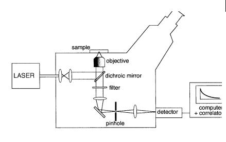
Most FCS instruments have been designed around optical microscopes. A typical optical configuration is shown in Figure 11.11. The emission is detected through a pinhole conjugated with the image plane of the excitation volume. The size of the latter depends on the magnification and pinhole size. The detector is a photomultiplier (or an avalanche photodiode) operating in the analog mode, or more often in single-photon counting mode, and is connected to an amplifier/discriminator. The autocorrelation function can be instantaneously obtained from the analysis of the fluorescence intensity fluctuations by a fast correlator. For the determination of rotational mobility, polarizers are introduced in the excitation and/ or emission path.

Two-photon FCS has been successfully developed; it o ers the advantage of 3-D resolution (see Section 11.2.1.2) (Chen et al., 2001).

11.3 Fluorescence correlation spectroscopy 367

Fig. 11.11. An optical microscope adapted for fluorescence correlation measurements.

11.3.2

Determination of translational di usion coe cients5)

For a single fluorescent species undergoing Brownian motion with a translational di usion coe cient Dt (see Chapter 8, Section 8.1), the autocorrelation function, in the case of Gaussian intensity distribution in the x; y plane and infinite dimension in the z-direction, is given by

where tD ¼ o2=4Dt is the characteristic time for di usion, and o is the distance from the center of the illuminated area in the x; y plane at which the detected fluorescence has dropped by a factor e2.

For a finite volume element with a Gaussian intensity distribution in three dimensions, the autocorrelation can be written as

where o1 and o2 are the distances from the center of the excitation volume in the radial and axial direction, respectively, at which the detected fluorescence has dropped by a factor e2.

368 11 Advanced techniques in fluorescence spectroscopy

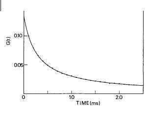
Fig. 11.12. Autocorrelation function for rhodamine 6G 10 9 M in ethanol. The best fit (solid line) yields Dt G3 10 6

cm2 s 1 (reproduced with permission from Thompson, 1991).

Translational di usion coe cients of fluorophores like rhodamine 6G have been determined by FCS and reasonable values of @3 10 6 cm2 s 1 were found (Figure 11.12). Tests with latex beads showed good agreement with known values.

Applications to fluorescent or fluorescently labeled proteins and nucleic acids, and to fluorescent lipid probes in phospholipid bilayers, have been reported. In the latter case, the di usion coe cients measured above the chain melting temperature were found to be A10 7 cm2 s 1, which is in agreement with values obtained by other techniques.

Translational di usion times of micelles can be measured by FCS, which allows calculation of the aggregation number (see Box 11.2).

Application of FCS to the determination of di usion coe cients of atoms in the gas phase has also been proposed.

11.3.3

Chemical kinetic studies

When translational di usion and chemical reactions are coupled, information can be obtained on the kinetic rate constants. Expressions for the autocorrelation function in the case of unimolecular and bimolecular reactions between states of di erent quantum yields have been obtained. In a general form, these expressions contain a large number of terms that reflect di erent combinations of di usion and reaction mechanisms.

In the case of complex formation, i.e. association–dissociation kinetics, there are two limiting cases of interest:

1.tchem ftD ¼ o2=4Dt: the chemical relaxation time is much smaller than the characteristic di usion time so that the equilibrium is reached during di usion through the excitation volume. Then, it su ces to replace the di usion coe - cient appearing in Eq. (11.8) by the weighted average hDti of the di usion co- e cients of the free and bound ligand:

11.3 Fluorescence correlation spectroscopy 369

Box 11.2 Determination of the size of micelles by FCS

The translational di usion coe cient of micelles loaded with a fluorophore can be determined from the autocorrelation function by means of Eqs (11.8) or (11.9). The hydrodynamic radius can then be calculated using the Stokes– Einstein relation (see Chapter 8, Section 8.1):

kT rh ¼ 6phDt

where k is the Boltzmann constant, T the temperature and h the viscosity (Pa s). Assuming that the micelles are spherical, the aggregation number, i.e. the number of surfactant molecules per micelle, is given by

4prr3Na n ¼ h

3m

where r is the mean density of the micelle (g cm 3), m is the molecular mass of a surfactant molecule (g mol 1) and Na is Avogadro’s number.

Figure B11.2.1 shows the normalized autocorrelation functions of various micelles loaded with octadecyl rhodamine B chloride (ODRB) at pH 7 (PBS bu er)a). The di erences in size of the micelles are clearly reflected by the differences in di usion times tD. The translational di usion coe cients are reported in Table B11.2.1, together with the hydrodynamic radii and the aggregation numbers.

Fig. B11.2.1. Autocorrelation curves for Rhodamine 6G and various micelles loaded with ODBR (reproduced with permission from Hink and Vissera)).

370 11 Advanced techniques in fluorescence spectroscopy

Tab. B11.2.1. Translational di usion coe cients, hydrodynamic volumes and aggregation numbers of various micelles loaded with ODRB

The di usion coe cients obtained with another fluorophore (NBD derivative) were slightly di erent. The values of the aggregations numbers were found to be often overestimated because incorporation of the fluorescent probe may require extra surfactant molecules. However, the relative size di erences between the micelles are in good agreement with the values reported in the literature. In addition to the size of micelles, FCS can give information on the size distribution.

a)Hink M. and Visser A. J. W. G. (1999) in: Rettig W. et al. (Eds), Applied Fluorescence in Chemistry, Biology and Medicine, SpringerVerlag, Berlin, pp. 101–18.

2.tchem gtD ¼ o2=4Dt: the chemical relaxation time is much larger than the characteristic di usion time so that there is no chemical exchange during diffusion through the excitation volume. The autocorrelation function is then given by

In both cases, the fractions of free and bound ligands can be determined provided that the di usion coe cients of these species are known.

11.3 Fluorescence correlation spectroscopy 371

Triplet state kinetics can also be studied by FCS (Widengren et al., 1995). In fact, with dyes such as fluoresceins and rhodamines, additional fluctuations in fluorescence are observed when increasing excitation intensities as the molecules enter and leave their triplet states. The time-dependent part of the autocorrelation function is given by

where GDðtÞ is the time-dependent part of the autocorrelation function for translational di usion (i.e. GðtÞ 1 obtained from Eqs 11.8 or 11.9), 3N is the average fraction of fluorophores within the sample volume element that are in their triplet state, and tT is the relaxation time from the triplet state. FCS is a convenient method for the determination of triplet parameters of fluorophores in solution. Because these parameters are sensitive to the fluorophore environment, FCS can be used for probing molecular microenvironments by monitoring triplet states.

Photoinduced electron transfer and photoisomerization can also be studied by FCS.

11.3.4

Determination of rotational di usion coe cients

When the excitation light is polarized and/or if the emitted fluorescence is detected through a polarizer, rotational motion of a fluorophore causes fluctuations in fluorescence intensity. We will consider only the case where the fluorescence decay, the rotational motion and the translational di usion are well separated in time. In other words, the relevant parameters are such that tS ftc ftD, where tS is the lifetime of the singlet excited state, tc is the rotational correlation time (defined as 1=6Dr where Dr is the rotational di usion coe cient; see Chapter 5, Section 5.6.1), and tD is the di usion time defined above. Then, the normalized autocorrelation function can be written as (Rigler et al., 1993)

This relation shows that the rotational correlation time is uncoupled from the excitedstate lifetime, in contrast to classical steady-state or time-resolved fluorescence polarization measurements (see Chapter 5). The important consequence is the possibility of observing slow rotations with fluorophores of short lifetime. This is the case for biological macromolecules labeled with fluorophores (e.g. rhodamine) whose lifetime is of a few nanoseconds.

Note that the translational di usion time decreases when the beam radius is decreased but not the rotational correlation time.

37211 Advanced techniques in fluorescence spectroscopy

11.4

Single-molecule fluorescence spectroscopy

11.4.1

General remarks

Since the pioneering work of Moerner and Kador in 1989 on doped crystals, singlemolecule detection has considerably expanded because it opens up new opportunities in analytical, material and biological sciences. For instance, sensitive detection is a major issue for the study of devices operating at a molecular level, and for observation of single biological macromolecules (tagged proteins or DNA). In bulk measurements, the properties of individual molecules are hidden in ensemble averages, whereas observation at the single molecule level provides new insights into physical, chemical and biological phenomena. New applications have emerged in analytical chemistry, biotechnology and the pharmaceutical industries.

The challenge in single-molecule detection is more a matter of background reduction than sensitive detection. In fact, single-photon detection techniques have long been used in spectroscopy, but the major di culty is detecting fluorescence photons on top of background photons arising from Rayleigh and Raman scattering and from fluorescence impurities.

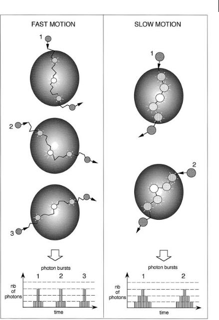
While a fluorescent molecule transits in a focused laser beam (during a few ms), it undergoes cycles of photon absorption and emission so that its presence is signaled by a burst of emitted photons, which allows us to distinguish the signal from background (Figure 11.13).

The point is now to estimate the maximum number of photons that can be detected from a burst. The maximum rate at which a molecule can emit is roughly the reciprocal of the excited-state lifetime. Therefore, the maximum number of photons emitted in a burst is approximately equal to the transit time divided by the excited-state lifetime. For a transit time of 1 ms and a lifetime of 1 ns, the maximum number is 106. However, photobleaching limits this number to about 105 photons for the most stable fluorescent molecules. The detection e ciency of specially designed optical systems with high numerical aperture being about 1%, we cannot expect to detect more than 1000 photons per burst. The background can be minimized by careful clean-up of the solvent and by using small excitation volumes (A1 pL in hydrodynamically focused sample streams, A1 fL in confocal excitation and detection with oneand two-photon excitation, and even smaller volumes with near-field excitation).

11.4.2

Single-molecule detection in flowing solutions

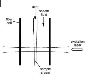
A small sample volume in a flowing solution can be obtained by introducing the sample from a capillary tube inserted into a flow cell (Ambrose et al., 1999) (Figure 11.14). This tube is surrounded by a rapidly flowing sheath fluid so that the sample stream is focused as it exits the capillary. The sample stream resulting from such

11.4 Single-molecule fluorescence spectroscopy 373

Fig. 11.13. Photon burst detection of single molecules in a focused laser beam.

hydrodynamic focusing has a diameter ranging from 1 to 20 mm. The laser beam is focused to a diameter of 10 mm. Typical sample volume elements are 1–10 pL.

The background resulting from Raman and Rayleigh scattering can be drastically reduced using a pulsed laser and the single-photon timing technique (see Chapter

374 11 Advanced techniques in fluorescence spectroscopy

Fig. 11.14. Principle of singlemolecule detection in flowing solutions (adapted from Goodwin et al., 1996, Acc. Chem. Res. 29, 607).

6, Section 6.2.2) as follows: because the excited-state lifetime is generally of a few nanoseconds, a single-channel analyzer is used in conjunction with a time-to- amplitude converter to process only the photons that are detected at times longer than 1 ns after the excitation pulse.

The single-photon timing technique has the additional advantage of providing an estimate of the excited-state lifetime from the histogram of arrival times of the photons on the detector. From the fluorescence decay of a single molecule of Rhodamine 110 (Figure 11.15), an excited-state lifetime of 3:9 G0:6 ns is estimated. Lifetime measurement is of interest for identification of single molecules.

Steady-state and time-resolved emission anisotropy measurements also allows distinction of single molecules on the basis of their rotational correlation time.

As far as applications are concerned, DNA sequencing has received much attention (see Box 11.3).

11.4.3

Single-molecule detection using advanced fluorescence microscopy techniques

Confocal microscopes (see Section 11.2.1.1) are well suited to the detection of single molecules. A photon burst is emitted when the molecule di uses through the excitation volume (0.1–1 fL). An example is given in Figure 11.16.

Single-molecule detection in confocal spectroscopy is characterized by an excellent signal-to-noise ratio, but the detection e ciency is in general very low because the excitation volume is very small with respect to the whole sample volume, and most molecules do not pass through the excitation volume. Moreover, the same molecule may re-enter this volume several times, which complicates data interpretation. Better detection e ciencies can be obtained by using microcapillaries and microstructures to force the molecules to enter the excitation volume. A nice example of the application of single-molecule detection with confocal microscopy is