Molecular Fluorescence

10.6 Towards fluorescence-based chemical sensing devices 335

Fig. 10.45. Examples of optical configurations for active optical sensors.

. In the active mode, the optical device uses for optical transduction the changes in the fluorescence characteristics of a fluorescent molecular sensor (as described in the preceding sections) resulting from the interaction with an analyte3). The two main optical configurations are:

1.In most cases, the fluorescent molecular sensor is immobilized at the tip of an optical fiber (active optode) in a matrix that permits di usion of the analyte (Figure 10.45). Plasticized polymers (e.g. polyvinyl chloride, PVC) and sol–gel glasses (e.g. SiO2 or TiO2) are often used as matrices. The advantage of the latter is the rapidity of the response. Various other methods have been used: grafting on silica, dextrins, cellulose, polymers (e.g. polystyrene, polyacrylamide), adsorption on membranes (e.g. polytetrafluoroethylene, PTFE), electrostatic coupling (with ion exchange membranes).

2.The second possibility is to make use of the continuous evanescent field that exists at the surface of an optical fiber. The cladding layer is replaced by a layer containing the fluorescent molecular sensor in a short portion of the optical fiber (Figure 10.45). At each reflection at the surface of the fiber core, the eva-

3)Alternatively, in some cases, the fluorophore chemically reacts with the analyte – these are outside the scope of this chapter.

336 10 Fluorescent molecular sensors of ions and molecules

nescent wave penetrates into the layer within a distance of the order of the wavelength of the propagating light. Fluorescence emitted within this evanescent region can be reciprocally coupled back into the core and conveyed towards the detector. Sensors using evanescent waves in planar waveguides have been also designed.

Various pH sensors have been built with a fluorescent pH indicator (fluorescein, eosin Y, pyranine, 4-methylumbelliferone, SNARF, carboxy-SNAFL) immobilized at the tip of an optical fiber. The response of a pH sensor corresponds to the titration curve of the indicator, which has a sigmoidal shape with an inflection point for pH ¼ pKa; but it should be emphasized that the e ective pKa value can be strongly influenced by the physical and chemical properties of the matrix in which the indicator is entrapped (or of the surface on which it is immobilized) without forgetting the dependence on temperature and ionic strength. In solution, the dynamic range is restricted to approximately two pH units, whereas it can be significantly extended (up to four units) when the indicator is immobilized in a microheterogeneous microenvironment (e.g. a sol–gel matrix).

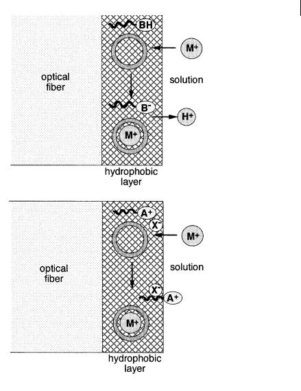
The same principle can be applied to cation sensors by using an immobilized fluoroionophore. An alternative is the use of neutral ion carriers coupled to a fluorescent co-reagent in a hydrophobic layer (e.g. plasticized PVC). The principle is based on the electroneutrality in the membrane, as illustrated in Figure 10.46. The first method employs a hydrophobic pH indicator dye as a co-reagent: when a cation is pulled into the hydrophobic layer by the neutral carrier (e.g. valinomycin for Kþ), the same number of Hþ must be released from the hydrophobic layer, and deprotonation of the pH indicator (whose role is to achieve proton exchange to maintain electroneutrality) is accompanied by a change in absorbance and fluorescence. In the second method, the co-reagent is an amphiphilic indicator possessing a hydrocarbon tail and a polar head that is a positively charged fluorescent group sensitive to polarity. Upon cation complexation in the layer by the neutral carrier, electroneutrality is maintained by partitioning out of the hydrophobic layer the polar head into the aqueous phase at the interface, which results in a change in fluorescence. The hydrophobic tail of the indicator prevents leaching.

Fluorescence-based gas sensors have been extensively developed. In particular, oxygen sensors are based on the dynamic quenching of a fluorophore (e.g. pyrene, pyrene butyric acid, complexes with Ru, Re, Pt) that is either entrapped in a matrix (e.g. porous glass, polymers like PVC, silicone layer) or adsorbed on a resin, or grafted on silica. For sensing acidic and basic gases such as ammonia, carbon dioxide, hydrogen cyanide or nitrogen oxide, a solution of a pH indicator (e.g. pyranine, fluorescein) is separated from the sample solution by a gas-permeable membrane (made of silicone or PTFE). The acidic or basic gas can cross the membrane and enter the solution containing the indicator, which undergoes proton tranfer. For further details on fluorescence-based chemical sensing devices, the reader is referred to specialized books and reviews (e.g. Arnold, 1992; Fuh et al., 1991; Janata, 1992; Seitz, 1984; Wolfbeis et al., 1988, 1991, 1996). It is beyond the scope of this chapter to describe biosensors.

10.6 Towards fluorescence-based chemical sensing devices 337

Fig. 10.46. Principles of optodes using a neutral carrier (e.g. valinomycin for Kþ) coupled to an amphiphilic fluorophore: (A) an amphiphilic pH indicator (Seiler K. et al. (1989) Anal. Sci. 5, 557). (B) a fluorescent cationic surfactant (e.g. dodecyl acridine orange) (Kawabata Y. et al. (1990) Anal. Chem. 62, 2054).

Appendix A. Spectrophotometric and spectrofluorometric pH titrations

Single-wavelength measurements

The concentration of the indicator is kept low enough that the linear relationship between aborbance or fluorescence intensity and concentration is fulfilled.

338 10 Fluorescent molecular sensors of ions and molecules

At a given wavelength, where both acidic form A and basic form B absorb or emit, the absorbance or the fluorescence intensity, denoted Y, are given by

In spectrophotometry, Y is the absorbance AðlÞ of the solution at the chosen wavelength l. According to the Beer–Lambert law, a and b are the products of the absorption pathlength by the molar absorption coe cients of A and B, respectively.

In spectrofluorometry, Y is the fluorescence intensity IFðlE; lFÞ of the solution for a couple of excitation and observation wavelengths. a and b are proportional to the molar absorption coe cients (at the excitation wavelength) and the fluorescence quantum yields of A and B, respectively.

When the indicator is only in the acidic form or only in the basic form, the values of Y are, respectively,

The value of pKa can thus be determined from the plot of log½ðY YAÞ=ðYB YAÞ& vs pH.

Dual-wavelength measurements

The absorbances or fluorescence intensities measured at two wavelengths l1 and l2 can be written in a form analogous to Eq. (A.1):

A ratiometric measurement consists of monitoring the ratio Yðl1Þ=Yðl2Þ given by

340 10 Fluorescent molecular sensors of ions and molecules

the thermodynamic point of view, the true equilibrium constant (which depends only on temperature) must be written with activities:

When the solution is dilute enough to approximate the activity coe cients to 1 (reference state: solute at infinite dilution), activities can then be replaced by molar fractions (dimensionless quantities), but in solution they are generally replaced by molar concentrations:

However, the equilibrium constant must still be considered as pure and dimensionless numbers (according to the classical relation DG0 ¼ RT ln Ks). All molar concentrations in the expression of Ks should thus be interpreted as molar concentrations relative to a standard state of 1 mol dm 3: i.e. they are the numerical values of the molar concentrations5). If the solution is not dilute enough, the equilibrium constants can still be written with concentrations but they must be considered as apparent stability constants.

When a second complex of stoichiometry 2:1 (metal:ligand) is formed, the following equilibria should be considered, assuming stepwise binding

M þ L Ð ML

ML þ M Ð M2L

The stepwise binding constants are defined as

It is possible to write the formation of the 2:1 complex directly from the cation and ligand as follows:

2M þ L Ð M2L

and to define an overall binding constant

Generalization to a complex MmLn can easily be made6):

mM þ lL Ð MmLl

Preliminary remarks on titrations by spectrophotometry and spectrofluorometry

In the following considerations, it will be assumed that the linear relationship between absorbance or fluorescence intensity and concentration is always fulfilled. Moreover, we will consider only the case where the ligand absorbs light or emits fluorescence but not the cation. In a titration experiment, the concentration of the ligand is kept constant and the metal salt is gradually added. The absorption spectrum or fluorescence spectrum is recorded as a function of cation concentration. Changes in these spectra upon complexation allow us to determine the stability constant of the complexes. Data can be processed using several wavelengths simultaneously. This may turn out to be necessary when several complexes are formed with overlap of their existence domains. This requires special software (a few are commercially available). However, when only one or two complexes exist, it may be su cient to monitor the variations in absorbance or fluorescence intensity at an appropriate wavelength (chosen so that the changes are as large as possible), or the variations in the ratio of absorbances or fluorescence intensities at two wavelengths. This is the subject of the following sections.

Formation of a 1:1 complex (single-wavelength measurements)

Let Y0 be the absorbance or the fluorescence intensity of the free ligand. In fluorometric experiments, the absorbance at the excitation wavelength should be less than @0.1. Then, at a given wavelength, Y0 is proportional to the concentration cL:

342 10 Fluorescent molecular sensors of ions and molecules

and in the presence of an excess of cation such that the ligand is fully complexed, Y reaches the limiting value Ylim:

In spectrophotometry, a and b are the products of the absorption pathlength by the molar absorption coe cients of the ligand and the complex, respectively. In spectrofluorometry, a and b are proportional to the molar absorption coe cients (at the excitation wavelength) and the fluorescent quantum yields of the ligand and the complex, respectively.

After addition of a given amount of cation at a concentration cM, the absorbance or the fluorescence intensity becomes

This relationship can be used to determine Ks under the condition that the concentration in free cation [M] can be approximated to the total concentration cM:

ðY Y0Þ=ðYlim YÞ is plotted as a function of cM, and the plot should be linear and the slope yields Ks. Once Ks is known, the concentration of free cation [M] can be determined by means of Eq. (B.13).

When Ylim is not measurable because full complexation cannot be attained at a reasonable concentration of cation, it is better to use the following relation:

where a ¼ a=ðb aÞ. It is convenient to plot Y0=ðY Y0Þ versus 1=cM provided that the approximation ½M&AcM is valid. The ratio of the ordinate at the origin to the slope yields Ks. Such a plot is called a double-reciprocal plot or a Benesi-Hildebrand plot.

The approximation ½M&AcM is made in most cases (Connors, 1987), and surprisingly little attention has been paid to cases where it is not valid (i.e. when KscL g1, see below). Yet an explicit expression of Y in the case of the formation of a 1:1 complex can be easily derived from the preceding equations without approximation. In fact, appropriate combinations of these equations lead to the following

10.6 Towards fluorescence-based chemical sensing devices 343

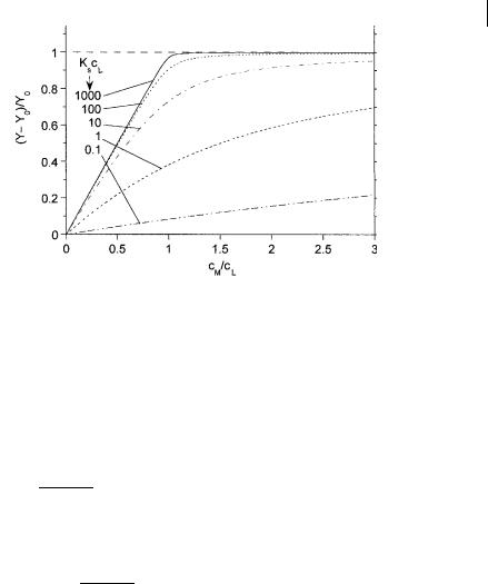
Fig. 10.B.1. Spectrophotometric or spectrofluorimetric titration curves for a complex 1:1 according to Eq. (B.16). Ylim is chosen to be equal to 2Y0.

second-order equation:

where

x ¼ Y Y0

Ylim Y0

Hence,

Ks can thus be obtained by a nonlinear least squares analysis of Y versus cM or cM=cL. If Ylim cannot be accurately determined, it can be left as a floating parameter in the analysis. Figure 10.B.1 shows the variations of ðY Y0Þ=Y0 versus cM=cL for Ylim ¼ 2Y0. Attention should be paid to the concentration of ligand cL with respect to 1=Ks. When KscL g1, the determination of Ks will be inaccurate because the titration curve, Y versus cM=cL, will essentially consist of two portions of straight lines. In fact, when KscL g1, Eq. (B.16) reduces to Y ¼ Y0 þ ðYlim Y0ÞcM=cL for cM=cL < 1 and Y ¼ Ylim for cM=cL b1. Another restriction for the ligand concentration should be recalled when fluorescence intensities are measured: the absorbance at the excitation wavelength should be less than @0.1. In contrast, in spectrophotometric experiments, absorbance can be measured up to 2–3. Figure 10.B.1

344 10 Fluorescent molecular sensors of ions and molecules

shows also that the smaller the value of KscL, the larger the excess of cation to be added to reach Ylim. It is often preferable to leave this parameter floating in the analysis.

Formation of a 1:1 complex (dual-wavelength measurements)

The absorbances or fluorescence intensities measured at two wavelengths l1 and l2 can be written in a form analogous to Eq. (B.10):

The ratiometric measurement consists of monitoring the ratio Yðl1Þ=Yðl2Þ given by

Taking into account Eqs (B.11) and (B.12), we obtain the following equation:

Note that a2=b2 represents the ratio of the absorbances or fluorescent intensities of the free ligand and the complex at the wavelength l2: a2=b2 ¼ Y0ðl2Þ=Ylimðl2Þ.

Equation (B.22) can be used for the determination of Ks only if the concentration in free cation [M] can be approximated to the total concentration cM.

When Ks is known, the concentration of free cation [M] can be determined by means of Eq. (B.22).

Formation of successive complexes ML and M2L

Let us consider a ligand that can bind successively two cations according to the equilibria