Molecular Fluorescence

356 11 Advanced techniques in fluorescence spectroscopy

excite a molecule that absorbs in the UV. Two-photon excitation is a nonlinear process; there is a quadratic dependence of absorption on excitation light intensity.

When a single laser is used, the two photons are of identical wavelength, and the technique is called two-photon excitation fluorescence microscopy. When the photons are of di erent wavelengths l1 and l2 (so that 1=l1 þ 1=l2 ¼ 1=le), the technique is called two-color excitation fluorescence microscopy.

The probability of two-photon absorption depends on both spatial and temporal overlap of the incident photons (the photons must arrive within 10 18 s). The crosssections for two-photon absorption are small, typically 10 50 cm4 s photon 1 molecule 1 for rhodamine B. Consequently, only fluorophores located in a region of very large photon flux can be excited. Mode-locked, high-peak power lasers like titanium–sapphire lasers can provide enough intensity for two-photon excitation in microscopy.

Because the excitation intensity varies as the square of the distance from the focal plane, the probability of two-photon absorption outside the focal region falls o with the fourth power of the distance along the z optical axis. Excitation of fluorophores can occur only at the point of focus. Using an objective with a numerical aperture of 1.25 and an excitation beam at 780 nm, over 80% of total fluorescence intensity is confined to within 1 mm of the focal plane. The excitation volume is of the order of 0.1–1 femtoliter. Compared to conventional fluorometers, this represents a reduction by a factor of 1010 of the excitation volume.

Two-photon excitation provides intrinsic 3-D resolution in laser scanning fluorescence microscopy. The 3-D sectioning e ect is comparable to that of confocal microscopy, but it o ers two advantages with respect to the latter: because the illumination is concentrated in both time and space, there is no out-of-focus photobleaching, and the excitation beam is not attenuated by out-of-focus absorption, which results in increased penetration depth of the excitation light.

The advantage of two-color excitation over two-photon excitation is not an improvement in imaging resolution, but the easier observation of microscopic objects through highly scattering media. In fact, in two-color excitation, scattering decreases the in-focus fluorescence but only minimally increases the unwanted fluorescence background, in contrast to two-photon excitation.

11.2.1.3 Near-field scanning optical microscopy (NSOM)

The resolution of a conventional microcope is limited by the classical phenomena of interference and di raction. The limit is approximately l=2, l being the wavelength. This limit can be overcome by using a sub-wavelength light source and by placing the sample very close to this source (i.e. in the near field). The relevant domain is near-field optics (as opposed to far-field conventional optics), which has been applied to microscopy, spectroscopy and optical sensors. In particular, nearfield scanning optical microscopy (NSOM) has proved to be a powerful tool in physical, chemical and life sciences (Dunn, 1999).

The idea of near-field optics to bypass the di raction limit was described in three visionary papers published by Synge in the period 1928–32. Synge’s idea is illus-

11.2 Advanced fluorescence microscopy 357

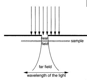
Fig. 11.5. Principle of nearfield optics according to Synge’s idea to overcome the diffraction limit.

trated in Figure 11.5. An incident light passes through a sub-wavelength hole in an opaque screen. The surface of the sample is positioned in close proximity to the hole so that the emerging light is forced to interact with it. The hole acts as a sub- wavelength-sized light probe that can be used to image a specimen before the light is di racted out. The first measurement using this idea was reported half a century later, and today NSOM is used in many fields. In addition to its very high spatial resolution at the sub-micrometer level, this technique has an outstanding sensitivity that permits single-molecule measurements (see Section 11.4.2).

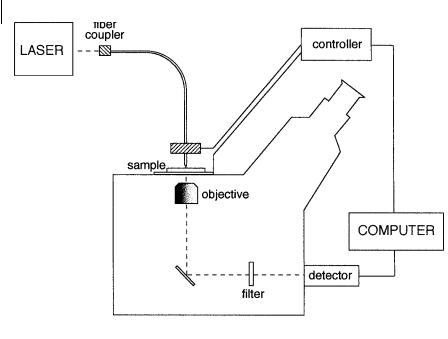
Most NSOM instruments are built around an inverted fluorescence microscope that o ers the advantage of providing normal images, allowing the region to be studied to be located with the higher resolution NSOM mode (Figure 11.6). A laser beam passes through a single mode optical fiber whose end is fashioned into a near-field tip. The tip is held in a z-piezo head. An x–y piezo stage on which the sample is mounted permits scanning of the sample. Light from the tip excites the sample whose emitted fluorescence is collected from below by an objective with a high numerical aperture and detected through a filter (to remove residual laser excitation light) and a detector (e.g. avalanche photodiode or OMA (optical multichannel analyzer)). This mode is called the illumination mode. Alternatively, in the collection mode, the sample is illuminated from the far field, and fluorescence is collected by the NSOM tip.

The systems that scan the piezos and record the image are similar to those used in atomic force microscopy.

The NSOM tip is obtained by heating and pulling a single-mode optical fiber down to a fine point. A reflective metal coating (aluminum, silver or gold) is deposited by vacuum evaporative techniques in order to prevent light from escaping.

Precise positioning of the tip within nanometers of the sample surface is required to obtain high-resolution images. This can be achieved by a feedback

358 11 Advanced techniques in fluorescence spectroscopy

Fig. 11.6. Schematic of an NSOM instrument built around an inverted fluorescence microscope and operating according to the illumination mode.

mechanism that is generally based on the shear-force method: the tip is dithered laterally at one of its resonating frequencies with an amplitude of about 2–5 nm. As the tip comes within the van der Waals force field of the sample, the shear forces dampen the amplitude of the tip vibration. This amplitude can be monitored and used to generate a feedback signal to control the distance between the sample and the tip during imaging.

NSOM is a remarkable tool for the analysis of thin films such as electroluminescent polymers (e.g. poly(p-phenylene vinylene), poly(p-pyridyl vinylene)), J- aggregates, liquid crystals and Langmuir–Blodgett films. Moreover, NSOM can provide new insights into complex biological systems owing to the higher resolution than in confocal microscopy, with the additional capability of force mapping of the surface topography, and the advantage of reduced photobleaching. Photosynthetic systems, protein localization, chromosome mapping and membrane microstructure are examples of systems that have been successfully investigated by NSOM. Imaging of fixed biological samples in aqueous environments is in fact possible, but the study of unfixed cells is problematic.

Discrimination of species in complex samples can be made via lifetime measurements using the single-photon timing method coupled to NSOM.

Two-photon excitation in NSOM has been shown to be possible with uncoated fiber tips in shared aperture arrangement. This represents an interesting extension of the technique to applications requiring UV light through two-photon excitation.

11.2 Advanced fluorescence microscopy 359

11.2.2

Fluorescence lifetime imaging microscopy (FLIM)

Fluorescence lifetime imaging uses di erences in the excited-state lifetime of fluorophores as a contrast mechanism for imaging. As emphasized in several chapters of this book, the excited-state lifetime of a fluorophore is sensitive to its microenvironment. Therefore, imaging of the lifetime provides complementary information on local physical parameters (e.g. microviscosity) and chemical parameters (e.g. pH, ion concentration), in addition to information obtained from steady-state characteristics (fluorescence spectra, excitation spectra and polarization). FLIM is an outstanding tool for the study of single cells with the possibility of coupling multi-parameter imaging of cellular structures with spectral information. Discrimination of autofluorescence of living cells from true fluorescence is possible on the basis of distinct lifetime di erences. Various applications have been reported: calcium (or other chemical) imaging; membrane fluidity, transport and fusion; imaging using RET (resonance energy transfer) for quantifying the distance between two species labelled with two di erent fluorophores; DNA sequencing; clinical imaging (e.g. use of antibodies and nucleic acids labeled with fluorophores for quantitative measurements of multiple disease markers in individual cells of patient specimens; etc.).

FLIM has been developed using either time-domain or frequency-domain methods (Herman et al., 1997).

11.2.2.1 Time-domain FLIM

In principle, lifetime imaging is possible by combination of the single-photon timing technique with scanning techniques. However, the long measurement time required for collecting photons at each point is problematic.

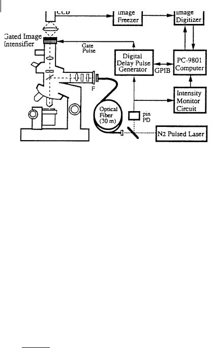
Alternatively, a gated microchannel plate (MCP) image intensifier (operating at a maximal frequency of 10 kHz) can be used in conjunction with a slow-scan cooled CCD camera for digital recording (Wang et al., 1992). Laser picosecond pulses are used to illuminate the entire field of view via an optical fiber and a lens of large numerical aperture (Figure 11.7).

The principle of lifetime measurement by the gated image intensifier is illustrated in Figure 11.8. At time td after excitation by a light pulse, a sampling gate pulse (duration DT) is applied to the photocathode of the image intensifier. Fluorescence can thus be detected at various delay times (multigate detection). For a single exponential decay of the form a expð t=tÞ, two delay times t1 and t2 are su cient. From corresponding fluorescence signals D1 and D2 given by

360 11 Advanced techniques in fluorescence spectroscopy

Fig. 11.7. A fluorescence lifetime microscope using a gated image intensifier (reproduced with permission from Wang et al., 1992).

Fig. 11.8. Principle of lifetime measurement by the gated image intensifier (adapted from Wang et al., 1992).

the lifetime can be calculated by means of the following expression:

(D1; D2; t1 and t2), lifetime images can be obtained very quickly. Time-resolved im-

11.2 Advanced fluorescence microscopy 361

ages can be accumulated on the CCD chip by repeated pulse excitation. The images are then read out to a computer.

The time resolution of the image intensifier is about 3 ns (minimal gate width), which may not be su cient for fast decaying probes. Moreover, a pixel-by-pixel deconvolution, if necessary, would require excessively long computation times.

A much better time resolution, together with space resolution, can be obtained by new imaging detectors consisting of a microchannel plate photomultiplier (MCP) in which the disk anode is replaced by a ‘coded’ anode (Kemnitz, 2001). Using a Ti–sapphire laser as excitation source and the single-photon timing method of detection, the time resolution is <10 ps. The space resolution is 100 mm (250 250 channels).

11.2.2.2 Frequency-domain FLIM

In frequency-domain FLIM, the optics and detection system (MCP image intensifier and slow scan CCD camera) are similar to that of time-domain FLIM, except for the light source, which consists of a CW laser and an acousto-optical modulator instead of a pulsed laser. The principle of lifetime measurement is the same as that described in Chapter 6 (Section 6.2.3.1). The phase shift and modulation depth are measured relative to a known fluorescence standard or to scattering of the excitation light. There are two possible modes of detection: heterodyne and homodyne detection.

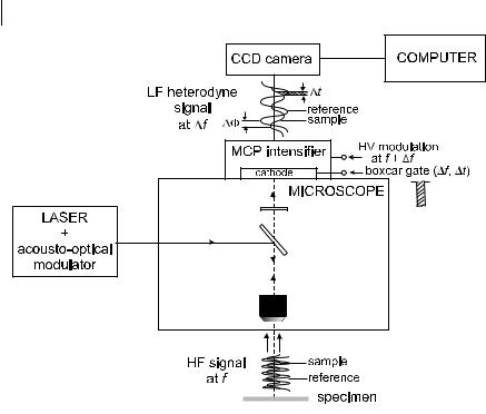
Heterodyne detection is achieved by modulating the high-voltage amplification of the image intensifier at frequency f þ Df , while fluorescence is modulated at frequency f . The high-frequency fluorescence signal is then transformed into a signal modulated at frequency Df (a few tens of Hz), which contains the same phase and modulation information as the original high-frequency signal. The phase and modulation of the Df signal are determined simultaneously at each pixel of the CCD camera. To do so, it is advantageous to use a ‘boxcar’ method of measurement by gating the cathode of the image intensifier for a time Dt repetitively and synchronously with the Df frequency master (Figure 11.9) (Gadella et al., 1993). Several phase delays settings are selected by systematically delaying the position of the gate. Separate images are recorded and accumulated on the CCD camera.

In the homodyne mode of detection, the modulation frequency of the excitation light is the same as that of the image intensifier. An example of data is shown in Box 11.1.

In the case of a single exponential decay, the lifetime can be rapidly calculated by either the phase shift F or the modulation ratio M by means of Eqs (6.25) and (6.26) established in Chapter 6 (Section 6.2.3):

362 11 Advanced techniques in fluorescence spectroscopy

Fig. 11.9. Schematic of phase measurement using a ‘boxcar’ method (adapted from Gadella et al., 1993).

If the values calculated in these two ways are identical, the fluorescence decay is indeed a single exponential. Otherwise, for a multi-component decay, tF < tM. In this case, several series of images have to be acquired at di erent frequencies (at least 5 for a triple exponential decay because three lifetimes and two fractional amplitudes are to be determined), which is a challenging computational problem.

11.2.2.3 Confocal FLIM (CFLIM)

As shown in Section 11.2.1.1, more details can be obtained by confocal fluorescence microscopy than by conventional fluorescence microscopy. In principle, the extension of conventional FLIM to confocal FLIM using either timeor frequencydomain methods is possible. However, the time-domain method based on singlephoton timing requires expensive lasers with high repetition rates to acquire an image in a reasonable time, because each pixel requires many photon events to generate a decay curve. In contrast, the frequency-domain method using an inexpensive CW laser coupled with an acoustooptic modulator is well suited to confocal FLIM.

11.2.2.4 Two-photon FLIM

As described above, two-photon excitation microscopy provides several advantages (reduced photobleaching, deeper penetration into the specimen). A fluorescence microscope combining two-photon excitation and fluorescence time-resolved

11.2 Advanced fluorescence microscopy 363

Box 11.1 An example of FLIM dataa)

A great deal of information is available when lifetimes are imaged. It is indispensable for the user to have as much information as possible presented in images and plots that convey multiple parameters simultaneously and conveniently, especially when the images are available in real time. The example presented in this box illustrates how to achieve this.

The data in Figure B11.1.1 were acquired with a frequency-domain FLIM instrument working in homodyne mode. In this mode, the modulation frequency of the intensifier (40 MHz) is identical to that of the excitation light (40 MHz). The phase and modulation are calculated from a series of images taken at different phase delays between the excitation light and the intensifier.

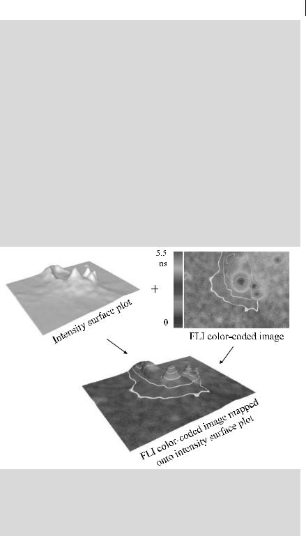
Figure B11.1.1 represents a 3T3 cell stained with BODIPY FL C5-ceramide (from Molecular Probes), a specific stain for the Golgi apparatus The color coding for the lifetimes is from 0 to 5 ns. The lifetime is coded in color (right upper) and this color-coded lifetime information is mapped onto the intensity surface (upper left) to give the combined lifetime/intensity plot (lower right). The final combined image shows intensity contours (in white), and a lit intensity surface is employed to accentuate the information in a three-dimensional form.

Fig. B11.1.1. FLIM data of a 3T3 cell (stained with BODIPY FL C5-ceramide) obtained by a frequency-domain FLIM instrument (see text)a).

a)Courtesy of Robert Clegg, Department of Physics, University of Illinois at UrbanaChampaign, USA.

364 11 Advanced techniques in fluorescence spectroscopy

imaging has been developed using a Ti:sapphire laser and the frequency-domain method with heterodyne detection (So et al., 1996). The Ti:sapphire laser is operated at a fixed frequency of 80 MHz. Because the pulse width is very narrow (150 fs), the train pulse has a harmonic content of up to 220 GHz. However, it is desirable to have modulation frequencies below 80 MHz in order to measure longer decay times. For this purpose, an acousto-optic modulator is placed in the beam path of the Ti:sapphire laser and provides modulation frequencies from 30 to 120 MHz. These frequencies are mixed with the 80 MHz repetition frequency of the laser and its high harmonics which generates new frequencies (sums and di erences). Finally, frequencies are available in the range of kilohertz to gigahertz.

11.3

Fluorescence correlation spectroscopy

In fluorescence correlation spectroscopy (FCS), the temporal fluctuations of the fluorescence intensity are recorded and analyzed in order to determine physical or chemical parameters such as translational di usion coe cients, flow rates, chemical kinetic rate constants, rotational di usion coe cients, molecular weights and aggregation. The principles of FCS for the determination of translational and rotational di usion and chemical reactions were first described in the early 1970s. But it is only in the early 1990s that progress in instrumentation (confocal excitation, photon detection and correlation) generated renewed interest in FCS.

11.3.1

Conceptual basis and instrumentation

Fluctuations in fluorescence intensity in a small open region (in general created by a focused laser beam) arise from the motion of fluorescent species in and out of this region via translational di usion or flow. Fluctuations can also arise from chemical reactions accompanied by a change in fluorescence intensity: association and dissociation of a complex, conformational transitions, photochemical reactions (Figure 11.10) (Thompson, 1991).

The fluctuations dIðtÞ of the fluorescence around the mean value hIi, defined as

are analyzed in the form of an autocorrelation function GðtÞ which relates the fluorescence intensity IðtÞ at time t to the fluorescence intensity Iðt þ tÞ at time t þ t:

ð11:7Þ