Biosignal and Biomedical Image Processing MATLAB based Applications - John L. Semmlow

FIGURE 11.7 A rotation transform using the nearest neighbor interpolation method. Pixel values in the output image (solid grid) are assigned values from the nearest pixel in the transformed input image (dashed grid).

more output pixels. In the bilinear interpolation method, the output pixel is the weighted average of transformed pixels in the nearest 2 by 2 neighborhood, and in bicubic interpolation the weighted average is taken over a 4 by 4 neighborhood.

Computational complexity and accuracy increase with the number of pixels that are considered in the interpolation, so there is a trade-off between quality and computational time. In MATLAB, the functions that require interpolation have an optional argument that specifies the method. For most functions, the default method is nearest neighbor. This method produces acceptable results on all image classes and is the only method appropriate for indexed images. The method is also the most appropriate for binary images. For RGB and intensity image classes, the bilinear or bicubic interpolation method is recommended since they lead to better results.

MATLAB provides several routines that can be used to generate a variety of complex spatial transformations such as image projections or specialized distortions. These transformations can be particularly useful when trying to overlay (register) images of the same structure taken at different times or with different modalities (e.g., PET scans and MRI images). While MATLAB’s spatial transformations routines allow for any imaginable transformation, only two types of transformation will be discussed here: affine transformations and projective transformations. Affine transformations are defined as transformations in which straight lines remain straight and parallel lines remain parallel, but rectangles may become parallelograms. These transformations include rotation, scaling, stretching, and shearing. In projective translations, straight lines still remain straight, but parallel lines often converge toward vanishing points. These transformations are discussed in the following MATLAB implementation section.

Copyright 2004 by Marcel Dekker, Inc. All Rights Reserved.

MATLAB Implementation

Affine Transformations

MATLAB provides a procedure described below for implementing any affine transformation; however, some of these transformations are so popular they are supported by separate routines. These include image resizing, cropping, and rotation. Image resizing and cropping are both techniques to change the dimensions of an image: the latter is interactive using the mouse and display while the former is under program control. To change the size of an image, MATLAB provides the ‘imresize’ command given below.

I_resize = imresize(I, arg or [M N], method);

where I is the original image and I_resize is the resized image. If the second argument is a scalar arg, then it gives a magnification factor, and if it is a vector, [M N], it indicates the desired new dimensions in vertical and horizontal pixels, M, N. If arg > 1, then the image is increased (magnified) in size proportionally and if arg < 1, it is reduced in size (minified). This will change image size proportionally. If the vector [M N] is used to specify the output size, image proportions can be modified: the image can be stretched or compressed along a given dimension. The argument method specifies the type of interpolation to be used and can be either ‘nearest’, ‘bilinear’, or ‘bicubic’, referring to the three interpolation methods described above. The nearest neighbor (nearest) is the default. If image size is reduced, then imresize automatically applies an antialiasing, lowpass filter unless the interpolation method is nearest; i.e., the default. The logic of this is that the nearest neighbor interpolation method would usually only be used with indexed images, and lowpass filtering is not really appropriate for these images.

Image cropping is an interactive command:

I_resize = imcrop;

The imcrop routine waits for the operator to draw an on-screen cropping rectangle using the mouse. The current image is resized to include only the image within the rectangle.

Image rotation is straightforward using the imrotate command:

I_rotate = imrotate(I, deg, method, bbox);

where I is the input image, I_rotate is the rotated image, deg is the degrees of rotation (counterclockwise if positive, and clockwise if negative), and method describes the interpolation method as in imresize. Again, the nearest neighbor

Copyright 2004 by Marcel Dekker, Inc. All Rights Reserved.

method is the default even though the other methods are preferred except for indexed images. After rotation, the image will not, in general, fit into the same rectangular boundary as the original image. In this situation, the rotated image can be cropped to fit within the original boundaries or the image size can be increased to fit the rotated image. Specifying the bbox argument as ‘crop’ will produce a cropped image having the dimensions of the original image, while setting bbox to ‘loose’ will produce a larger image that contains the entire original, unrotated, image. The loose option is the default. In either case, additional pixels will be required to fit the rotated image into a rectangular space (except for orthogonal rotations), and imrotate pads these with zeros producing a black background to the rotated image (see Figure 11.8).

Application of the imresize and imrotate routines is shown in Example 11.5 below. Application of imcrop is presented in one of the problems at the end of this chapter.

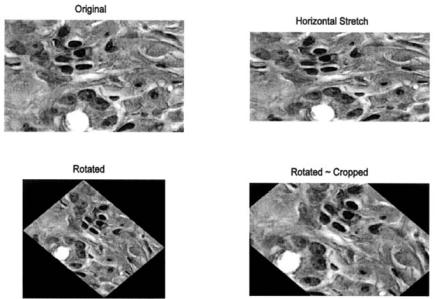
FIGURE 11.8 Two spatial transformations (horizontal stretching and rotation) applied to an image of bone marrow. The rotated images are cropped either to include the full image (lower left), or to have the same dimensions are the original image (lower right). Stained image courtesy of Alan W. Partin, M.D., Ph.D., Johns Hopkins University School of Medicine.

Copyright 2004 by Marcel Dekker, Inc. All Rights Reserved.

Example 11.5 Demonstrate resizing and rotation spatial transformations. Load the image of stained tissue (hestain.png) and transform it so that the horizontal dimension is 25% longer than in the original, keeping the vertical dimension unchanged. Rotate the original image 45 degrees clockwise, with and without cropping. Display the original and transformed images in a single figure.

%Example 11.5 and Figure 11.8

%Example of various Spatial Transformations

%Input the image of bone marrow (bonemarr.tif) and perform

%two spatial transformations:

%1) Stretch the object by 25% in the horizontal direction;

%2) Rotate the image clockwise by 30 deg. with and without

%cropping.

%Display the original and transformed images.

%

.......read image and convert if necessary .......

%

%Rotate image with and without cropping I_rotate = imrotate(I,-45, ’bilinear’);

I_rotate_crop = imrotate (I, -45, ’bilinear’, ’crop’);

[M N] = size(I);

%Stretch by 25% horin.

I_stretch = imresize (I,[M N*1.25], ’bilinear’);

%

.......display the images .........

The images produced by this code are shown in Figure 11.8.

General Affine Transformations

In the MATLAB Image Processing Toolbox, both affine and projective spatial transformations are defined by a Tform structure which is constructed using one of two routines: the routine maketform uses parameters supplied by the user to construct the transformation while cp2tform uses control points, or landmarks, placed on different images to generate the transformation. Both routines are very flexible and powerful, but that also means they are quite involved. This section describes aspects of the maketform routine, while the cp2tfrom routine will be presented in context with image registration.

Irrespective of the way in which the desired transformation is specified, it is implemented using the routine imtransform. This routine is only slightly less complicated than the transformation specification routines, and only some of its features will be discussed here. (The associated help file should be consulted for more detail.) The basic calling structure used to implement the spatial transformation is:

Copyright 2004 by Marcel Dekker, Inc. All Rights Reserved.

B = imtransform(A, Tform, ‘Param1’, value1, ‘Param2’,

value2,....);

where A and B are the input and output arrays, respectively, and Tform provides the transformation specifications as generated by maketform or cp2tform. The additional arguments are optional. The optional parameters are specified as pairs of arguments: a string containing the name of the optional parameter (i.e., ‘Param1’) followed by the value.* These parameters can (1) specify the pixels to be used from the input image (the default is the entire image), (2) permit a change in pixel size, (3) specify how to fill any extra background pixels generated by the transformation, and (4) specify the size and range of the output array. Only the parameters that specify output range will be discussed here, as they can be used to override the automatic rescaling of image size performed by imtransform. To specify output image range and size, parameters ‘XData’ and ‘YData’ are followed by a two-variable vector that gives the x or y coordinates of the first and last elements of the output array, B. To keep the size and range in the output image the same as the input image, simply specify the horizontal and vertical size of the input array, i.e.:

[M N] = size(A);

...

B = imtransform(A, Tform, ‘Xdata’, [1 N], ‘Ydata’, [1 M]);

As with the transform specification routines, imtransform uses the spatial coordinate system described at the beginning of the Chapter 10. In this system, the first dimension is the x coordinate while the second is the y, the reverse of the matrix subscripting convention used by MATLAB. (However the y coordinate still increases in the downward direction.) In addition, non-integer values for x and y indexes are allowed.

The routine maketform can be used to generate the spatial transformation descriptor, Tform. There are two alternative approaches to specifying the transformation, but the most straightforward uses simple geometrical objects to define the transformation. The calling structure under this approach is:

Tform = maketform(‘type’, U, X);

where ‘type’ defines the type of transformation and U and X are vectors that define the specific transformation by defining the input (U) and output (X) geometries. While maketform supports a variety of transformation types, including

*This is a common approach used in many MATLAB routines when a large number of arguments are possible, especially when many of these arguments are optional. It allows the arguments to be specified in any order.

Copyright 2004 by Marcel Dekker, Inc. All Rights Reserved.

custom, user-defined types, only the affine and projective transformations will be discussed here. These are specified by the type parameters ‘affine’ and

‘projective’.

Only three points are required to define an affine transformation, so, for this transformation type, U and X define corresponding vertices of input and output triangles. Specifically, U and X are 3 by 2 matrices where each 2-column row defines a corresponding vertex that maps input to output geometry. For example, to stretch an image vertically, define an output triangle that is taller than the input triangle. Assuming an input image of size M by N, to increase the vertical dimension by 50% define input (U) and output (X) triangles as:

U = [1, 1; 1, M; N, M]’ X = [1, 1-.5M; 1, M; N, M];

In this example, the input triangle, U, is simply the upper left, lower left, and lower right corners of the image. The output triangle, X, has its top, left vertex increased by 50%. (Recall the coordinate pairs are given as x,y and y increases negatively. Note that negative coordinates are acceptable). To increase the vertical dimension symmetrically, change X to:

X = [1, 1-.25M; 1, 1.25*M; N, 1.25*M];

In this case, the upper vertex is increased by only 25%, and the two lower vertexes are lowered in the y direction by increasing the y coordinate value by 25%. This transformation could be done with imresize, but this would also change the dimension of the output image. When this transform is implemented with imtransform, it is possible to control output size as described below. Hence this approach, although more complicated, allows greater control of the transformation. Of course, if output image size is kept the same, the contents of the original image, when stretched, may exceed the boundaries of the image and will be lost. An example of the use of this approach to change image proportions is given in Problem 6.

The maketform routine can be used to implement other affine transformations such as shearing. For example, to shear an image to the left, define an output triangle that is skewed by the desired amount with respect to the input triangle, Figure 11.9. In Figure 11.9, the input triangle is specified as: U = [N/ 2 1; 1 M; N M], (solid line) and the output triangle as X = [1 1; 1 M; N M] (solid line). This shearing transform is implemented in Example 11.6.

Projective Transformations

In projective transformations, straight lines remain straight but parallel lines may converge. Projective transformations can be used to give objects perspective. Projective transformations require four points for definition; hence, the

Copyright 2004 by Marcel Dekker, Inc. All Rights Reserved.

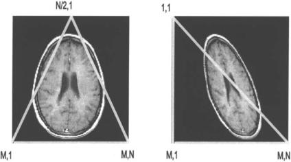
FIGURE 11.9 An affine transformation can be defined by three points. The transformation shown here is defined by an input (left) and output (right) triangle and produces a sheared image. M,N are indicated in this figure as row, column, but are actually specified in the algorithm in reverse order, as x,y. (Original image from the MATLAB Image Processing Toolbox. Copyright 1993–2003, The Math Work, Inc. Reprinted with permission.)

defining geometrical objects are quadrilaterals. Figure 11.10 shows a projective transformation in which the original image would appear to be tilted back. In this transformation, vertical lines in the original image would converge in the transformed image. In addition to adding perspective, these transformations are of value in correcting for relative tilts between image planes during image registration. In fact, most of these spatial transformations will be revisited in the section on image registration. Example 11.6 illustrates the use of these general image transformations for affine and projective transformations.

Example 11.6 General spatial transformations. Apply the affine and projective spatial transformation to one frame of the MRI image in mri.tif. The affine transformation should skew the top of the image to the left, just as shown in Figure 11.9. The projective transformation should tilt the image back as shown in Figure 11.10. This example will also use projective transformation to tilt the image forward, or opposite to that shown in Figure 11.10.

After the image is loaded, the affine input triangle is defined as an equilateral triangle inscribed within the full image. The output triangle is defined by shifting the top point to the left side, so the output triangle is now a right triangle (see Figure 11.9). In the projective transformation, the input quadrilateral is a

Copyright 2004 by Marcel Dekker, Inc. All Rights Reserved.

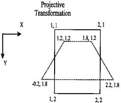
FIGURE 11.10 Specification of a projective transformation by defining two quadrilaterals. The solid lines define the input quadrilateral and the dashed line defines the desired output quadrilateral.

rectangle the same size as the input image. The output quadrilateral is generated by moving the upper points inward and down by an equal amount while the lower points are moved outward and up, also by a fixed amount. The second projective transformation is achieved by reversing the operations performed on the corners.

%Example 11.6 General Spatial Transformations

%Load a frame of the MRI image (mri.tif)

%and perform two spatial transformations

%1) An affine transformation that shears the image to the left

%2) A projective transformation that tilts the image backward

%3) A projective transformation that tilts the image forward clear all; close all;

%.......load frame 18 .......

%

% Define affine transformation

% Generate transform

Tform1 = maketform(’affine’, U1, X1);

% Apply transform

I_affine = imtransform(I, Tform1,’Size’, [M N]);

%

% Define projective transformation vectors

Copyright 2004 by Marcel Dekker, Inc. All Rights Reserved.

X = [1-offset 1 offset; 1 offset M-offset; ...

N-offset M-offset; N offset 1 offset];

%

%Define transformation based on vectors U and X Tform2 = maketform(’projective’, U, X);

I_proj1 = imtransform(I,Tform2,’Xdata’,[1 N],’Ydata’, ...

[1 M]);

%Second transformation. Define new output quadrilateral

X = [1 offset 1 offset; 1-offset M-offset; ...

N offset M-offset; N-offset 1 offset];

% Generate transform

Tform3 = maketform(’projective’, U, X);

% Apply transform

I_proj2 = imtransform(I,Tform3, ’Xdata’,[1 N],

’Ydata’,[1 M]);

%

.......display images .......

The images produced by this code are shown in Figure 11.11.

Of course, a great many other transforms can be constructed by redefining the output (or input) triangles or quadrilaterals. Some of these alternative transformations are explored in the problems.

All of these transforms can be applied to produce a series of images having slightly different projections. When these multiple images are shown as a movie, they will give an object the appearance of moving through space, perhaps in three dimensions. The last three problems at the end of this chapter explore these features. The following example demonstrates the construction of such a movie.

Example 11.7 Construct a series of projective transformations, that when shown as a movie, give the appearance of the image tilting backward in space. Use one of the frames of the MRI image.

Solution The code below uses the projective transformation to generate a series of images that appear to tilt back because of the geometry used. The approach is based on the second projective transformation in Example 11.7, but adjusts the transformation to produce a slightly larger apparent tilt in each frame. The program fills 24 frames in such a way that the first 12 have increasing angles of tilt and the last 12 frames have decreasing tilt. When shown as a movie, the image will appear to rock backward and forward. This same approach will also be used in Problem 7. Note that as the images are being generated by imtransform, they are converted to indexed images using gray2ind since this is the format required by immovie. The grayscale map generated by gray2ind is used (at the default level of 64), but any other map could be substituted in immovie to produce a pseudocolor image.

Copyright 2004 by Marcel Dekker, Inc. All Rights Reserved.

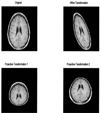
FIGURE 11.11 Original MR image and three spatial transformations. Upper right: An affine transformation that shears the image to the left. Lower left: A projective transform in which the image is made to appear tilted forward. Lower right: A projective transformation in which the image is made to appear tilted backward. (Original image from the MATLAB Image Processing Toolbox, Copyright 1993– 2003, The Math Works, Inc. Reprinted with permission.)

%Example 11.7 Spatial Transformation movie

%Load a frame of the MRI image (mri.tif). Use the projective

%transformation to make a movie of the image as it tilts

%horizontally.

........load MRI frame 12 as in previous examples .......

Copyright 2004 by Marcel Dekker, Inc. All Rights Reserved.