

- •List of Tables
- •List of Figures
- •Table of Notation
- •Preface
- •Boolean retrieval
- •An example information retrieval problem
- •Processing Boolean queries
- •The extended Boolean model versus ranked retrieval
- •References and further reading
- •The term vocabulary and postings lists
- •Document delineation and character sequence decoding
- •Obtaining the character sequence in a document
- •Choosing a document unit
- •Determining the vocabulary of terms
- •Tokenization
- •Dropping common terms: stop words
- •Normalization (equivalence classing of terms)
- •Stemming and lemmatization
- •Faster postings list intersection via skip pointers
- •Positional postings and phrase queries
- •Biword indexes
- •Positional indexes
- •Combination schemes
- •References and further reading
- •Dictionaries and tolerant retrieval
- •Search structures for dictionaries
- •Wildcard queries
- •General wildcard queries
- •Spelling correction
- •Implementing spelling correction
- •Forms of spelling correction
- •Edit distance
- •Context sensitive spelling correction
- •Phonetic correction
- •References and further reading
- •Index construction
- •Hardware basics
- •Blocked sort-based indexing
- •Single-pass in-memory indexing
- •Distributed indexing
- •Dynamic indexing
- •Other types of indexes
- •References and further reading
- •Index compression
- •Statistical properties of terms in information retrieval
- •Dictionary compression
- •Dictionary as a string
- •Blocked storage
- •Variable byte codes
- •References and further reading
- •Scoring, term weighting and the vector space model
- •Parametric and zone indexes
- •Weighted zone scoring
- •Learning weights
- •The optimal weight g
- •Term frequency and weighting
- •Inverse document frequency
- •The vector space model for scoring
- •Dot products
- •Queries as vectors
- •Computing vector scores
- •Sublinear tf scaling
- •Maximum tf normalization
- •Document and query weighting schemes
- •Pivoted normalized document length
- •References and further reading
- •Computing scores in a complete search system
- •Index elimination
- •Champion lists
- •Static quality scores and ordering
- •Impact ordering
- •Cluster pruning
- •Components of an information retrieval system
- •Tiered indexes
- •Designing parsing and scoring functions
- •Putting it all together
- •Vector space scoring and query operator interaction
- •References and further reading
- •Evaluation in information retrieval
- •Information retrieval system evaluation
- •Standard test collections
- •Evaluation of unranked retrieval sets
- •Evaluation of ranked retrieval results
- •Assessing relevance
- •A broader perspective: System quality and user utility
- •System issues
- •User utility
- •Results snippets
- •References and further reading
- •Relevance feedback and query expansion
- •Relevance feedback and pseudo relevance feedback
- •The Rocchio algorithm for relevance feedback
- •Probabilistic relevance feedback
- •When does relevance feedback work?
- •Relevance feedback on the web
- •Evaluation of relevance feedback strategies
- •Pseudo relevance feedback
- •Indirect relevance feedback
- •Summary
- •Global methods for query reformulation
- •Vocabulary tools for query reformulation
- •Query expansion
- •Automatic thesaurus generation
- •References and further reading
- •XML retrieval
- •Basic XML concepts
- •Challenges in XML retrieval
- •A vector space model for XML retrieval
- •Evaluation of XML retrieval
- •References and further reading
- •Exercises
- •Probabilistic information retrieval
- •Review of basic probability theory
- •The Probability Ranking Principle
- •The 1/0 loss case
- •The PRP with retrieval costs
- •The Binary Independence Model
- •Deriving a ranking function for query terms
- •Probability estimates in theory
- •Probability estimates in practice
- •Probabilistic approaches to relevance feedback
- •An appraisal and some extensions
- •An appraisal of probabilistic models
- •Bayesian network approaches to IR
- •References and further reading
- •Language models for information retrieval
- •Language models
- •Finite automata and language models
- •Types of language models
- •Multinomial distributions over words
- •The query likelihood model
- •Using query likelihood language models in IR
- •Estimating the query generation probability
- •Language modeling versus other approaches in IR
- •Extended language modeling approaches
- •References and further reading
- •Relation to multinomial unigram language model
- •The Bernoulli model
- •Properties of Naive Bayes
- •A variant of the multinomial model
- •Feature selection
- •Mutual information
- •Comparison of feature selection methods
- •References and further reading
- •Document representations and measures of relatedness in vector spaces
- •k nearest neighbor
- •Time complexity and optimality of kNN
- •The bias-variance tradeoff
- •References and further reading
- •Exercises
- •Support vector machines and machine learning on documents
- •Support vector machines: The linearly separable case
- •Extensions to the SVM model
- •Multiclass SVMs
- •Nonlinear SVMs
- •Experimental results
- •Machine learning methods in ad hoc information retrieval
- •Result ranking by machine learning
- •References and further reading
- •Flat clustering
- •Clustering in information retrieval
- •Problem statement
- •Evaluation of clustering
- •Cluster cardinality in K-means
- •Model-based clustering
- •References and further reading
- •Exercises
- •Hierarchical clustering
- •Hierarchical agglomerative clustering
- •Time complexity of HAC
- •Group-average agglomerative clustering
- •Centroid clustering
- •Optimality of HAC
- •Divisive clustering
- •Cluster labeling
- •Implementation notes
- •References and further reading
- •Exercises
- •Matrix decompositions and latent semantic indexing
- •Linear algebra review
- •Matrix decompositions
- •Term-document matrices and singular value decompositions
- •Low-rank approximations
- •Latent semantic indexing
- •References and further reading
- •Web search basics
- •Background and history
- •Web characteristics
- •The web graph
- •Spam
- •Advertising as the economic model
- •The search user experience
- •User query needs
- •Index size and estimation
- •Near-duplicates and shingling
- •References and further reading
- •Web crawling and indexes
- •Overview
- •Crawling
- •Crawler architecture
- •DNS resolution
- •The URL frontier
- •Distributing indexes
- •Connectivity servers
- •References and further reading
- •Link analysis
- •The Web as a graph
- •Anchor text and the web graph
- •PageRank
- •Markov chains
- •The PageRank computation
- •Hubs and Authorities
- •Choosing the subset of the Web
- •References and further reading
- •Bibliography
- •Author Index

356 |
16 Flat clustering |
a search problem. The brute force solution would be to enumerate all possible clusterings and pick the best. However, there are exponentially many partitions, so this approach is not feasible.1 For this reason, most flat clustering algorithms refine an initial partitioning iteratively. If the search starts at an unfavorable initial point, we may miss the global optimum. Finding a good starting point is therefore another important problem we have to solve in flat clustering.
16.3Evaluation of clustering
INTERNAL CRITERION OF QUALITY
EXTERNAL CRITERION OF QUALITY
PURITY
Typical objective functions in clustering formalize the goal of attaining high intra-cluster similarity (documents within a cluster are similar) and low intercluster similarity (documents from different clusters are dissimilar). This is an internal criterion for the quality of a clustering. But good scores on an internal criterion do not necessarily translate into good effectiveness in an application. An alternative to internal criteria is direct evaluation in the application of interest. For search result clustering, we may want to measure the time it takes users to find an answer with different clustering algorithms. This is the most direct evaluation, but it is expensive, especially if large user studies are necessary.
As a surrogate for user judgments, we can use a set of classes in an evaluation benchmark or gold standard (see Section 8.5, page 164, and Section 13.6, page 279). The gold standard is ideally produced by human judges with a good level of inter-judge agreement (see Chapter 8, page 152). We can then compute an external criterion that evaluates how well the clustering matches the gold standard classes. For example, we may want to say that the optimal clustering of the search results for jaguar in Figure 16.2 consists of three classes corresponding to the three senses car, animal, and operating system. In this type of evaluation, we only use the partition provided by the gold standard, not the class labels.
This section introduces four external criteria of clustering quality. Purity is a simple and transparent evaluation measure. Normalized mutual information can be information-theoretically interpreted. The Rand index penalizes both false positive and false negative decisions during clustering. The F measure in addition supports differential weighting of these two types of errors.
To compute purity, each cluster is assigned to the class which is most frequent in the cluster, and then the accuracy of this assignment is measured by counting the number of correctly assigned documents and dividing by N.
1. An upper bound on the number of clusterings is KN /K!. The exact number of different partitions of N documents into K clusters is the Stirling number of the second kind. See
http://mathworld.wolfram.com/StirlingNumberoftheSecondKind.html or Comtet (1974).
Online edition (c) 2009 Cambridge UP

16.3 Evaluation of clustering |
|
|
|
357 |
|
cluster 1 |
|
cluster 2 |
cluster 3 |
||
x |
x |
x |
o |
x |
|
o |
|
|
|||
x |
o o |
|
|
||
x |
x |
|
o |
|
x |
Figure 16.4 Purity as an external evaluation criterion for cluster quality. Majority class and number of members of the majority class for the three clusters are: x, 5 (cluster 1); o, 4 (cluster 2); and , 3 (cluster 3). Purity is (1/17) × (5 + 4 + 3) ≈ 0.71.
|
purity |
NMI |
RI |
F5 |
lower bound |
0.0 |
0.0 |
0.0 |
0.0 |
maximum |
1 |
1 |
1 |
1 |
value for Figure 16.4 |
0.71 |
0.36 |
0.68 |
0.46 |
Table 16.2 The four external evaluation measures applied to the clustering in Figure 16.4.
|
Formally: |
|
||
(16.1) |
purity(Ω, C) = |
1 |
∑ maxj |
|ωk ∩ cj| |
N |
||||
|
|
|
k |
|
|
where Ω = {ω1, ω2, . . . , ωK} is the set of clusters and C = {c1, c2, . . . , cJ} is |
|||
|
the set of classes. We interpret ωk as the set of documents in ωk and cj as the |
|||
|
set of documents in cj in Equation (16.1). |
|
||
|
We present an example of how to compute purity in Figure 16.4.2 Bad |
|||
|
clusterings have purity values close to 0, a perfect clustering has a purity of |
|||
|
1. Purity is compared with the other three measures discussed in this chapter |
|||
|
in Table 16.2. |
|
||
|
High purity is easy to achieve when the number of clusters is large – in |
|||
|
particular, purity is 1 if each document gets its own cluster. Thus, we cannot |
|||
|
use purity to trade off the quality of the clustering against the number of |
|||
|
clusters. |
|
||
NORMALIZED MUTUAL |
A measure that allows us to make this tradeoff is normalized mutual infor- |
|||
INFORMATION |
|
|
|
|
2. Recall our note of caution from Figure 14.2 (page 291) when looking at this and other 2D figures in this and the following chapter: these illustrations can be misleading because 2D projections of length-normalized vectors distort similarities and distances between points.
Online edition (c) 2009 Cambridge UP

358
(16.2)
(16.3)
(16.4)
(16.5)
(16.6)
16 Flat clustering
mation or NMI: |
I(Ω; C) |
|
NMI(Ω, C) = |
||
|
||
[H(Ω) + H(C)]/2 |
I is mutual information (cf. Chapter 13, page 272):
I(Ω; C) = ∑ ∑
k j
= ∑ ∑
k j
P(ωk ∩ cj)
P(ωk ∩ cj) log P(ωk)P(cj)
|ωk ∩ cj| log N|ωk ∩ cj| N |ωk||cj|
where P(ωk), P(cj), and P(ωk ∩ cj) are the probabilities of a document being in cluster ωk, class cj, and in the intersection of ωk and cj, respectively. Equation (16.4) is equivalent to Equation (16.3) for maximum likelihood estimates of the probabilities (i.e., the estimate of each probability is the corresponding relative frequency).
H is entropy as defined in Chapter 5 (page 99):
H(Ω) = |
− ∑ P(ωk) log P(ωk) |
|||
|
k |
|
|
|
= |
− ∑ |
|ωk| |
log |
|ωk| |
|
N |
|
N |
|
|
k |
|
|
|
where, again, the second equation is based on maximum likelihood estimates of the probabilities.
I(Ω; C) in Equation (16.3) measures the amount of information by which our knowledge about the classes increases when we are told what the clusters are. The minimum of I(Ω; C) is 0 if the clustering is random with respect to class membership. In that case, knowing that a document is in a particular cluster does not give us any new information about what its class might be. Maximum mutual information is reached for a clustering Ωexact that perfectly
recreates the classes – but also if clusters in Ωexact are further subdivided into smaller clusters (Exercise 16.7). In particular, a clustering with K = N one-
document clusters has maximum MI. So MI has the same problem as purity: it does not penalize large cardinalities and thus does not formalize our bias that, other things being equal, fewer clusters are better.
The normalization by the denominator [H(Ω) + H(C)]/2 in Equation (16.2) fixes this problem since entropy tends to increase with the number of clusters. For example, H(Ω) reaches its maximum log N for K = N, which ensures that NMI is low for K = N. Because NMI is normalized, we can use it to compare clusterings with different numbers of clusters. The particular form of the denominator is chosen because [H(Ω) + H(C)]/2 is a tight upper bound on I(Ω; C) (Exercise 16.8). Thus, NMI is always a number between 0 and 1.
Online edition (c) 2009 Cambridge UP
RAND INDEX
RI
F MEASURE
16.3 Evaluation of clustering |
359 |
An alternative to this information-theoretic interpretation of clustering is to view it as a series of decisions, one for each of the N(N − 1)/2 pairs of documents in the collection. We want to assign two documents to the same cluster if and only if they are similar. A true positive (TP) decision assigns two similar documents to the same cluster, a true negative (TN) decision assigns two dissimilar documents to different clusters. There are two types of errors we can commit. A false positive (FP) decision assigns two dissimilar documents to the same cluster. A false negative (FN) decision assigns two similar documents to different clusters. The Rand index (RI) measures the percentage of decisions that are correct. That is, it is simply accuracy (Section 8.3, page 155).
RI = |
TP + TN |
TP + FP + FN + TN |
As an example, we compute RI for Figure 16.4. We first compute TP + FP. The three clusters contain 6, 6, and 5 points, respectively, so the total number of “positives” or pairs of documents that are in the same cluster is:
TP + FP = |
2 |
+ |
2 |
+ |
2 |
= 40 |
|
6 |
|
6 |
|
5 |
|
Of these, the x pairs in cluster 1, the o pairs in cluster 2, the pairs in cluster 3, and the x pair in cluster 3 are true positives:
TP = |
2 |
+ |
2 |
+ |
2 |
+ |
2 |
= 20 |
|
5 |
|
4 |
|
3 |
|
2 |
|
Thus, FP = 40 − 20 = 20.
FN and TN are computed similarly, resulting in the following contingency
table: |
|
|
|
Same cluster |
Different clusters |
Same class |
TP = 20 |
FN = 24 |
Different classes |
FP = 20 |
TN = 72 |
RI is then (20 + 72)/(20 + 20 + 24 + 72) ≈ 0.68.
The Rand index gives equal weight to false positives and false negatives. Separating similar documents is sometimes worse than putting pairs of dissimilar documents in the same cluster. We can use the F measure (Section 8.3, page 154) to penalize false negatives more strongly than false positives by selecting a value β > 1, thus giving more weight to recall.
P = |
TP |
R = |
TP |
F = |
(β2 |
+ 1)PR |
||
|
|
|
|
|
|
|||
|
TP + FP |
|
TP + FN |
β |
β2 P + R |
|||
|
|
|
||||||
Online edition (c) 2009 Cambridge UP

360 |
16 Flat clustering |
Based on the numbers in the contingency table, P = 20/40 = 0.5 and R = 20/44 ≈ 0.455. This gives us F1 ≈ 0.48 for β = 1 and F5 ≈ 0.456 for β = 5. In information retrieval, evaluating clustering with F has the advantage that the measure is already familiar to the research community.
?Exercise 16.3
Replace every point d in Figure 16.4 with two identical copies of d in the same class.
(i)Is it less difficult, equally difficult or more difficult to cluster this set of 34 points
as opposed to the 17 points in Figure 16.4? (ii) Compute purity, NMI, RI, and F5 for the clustering with 34 points. Which measures increase and which stay the same after doubling the number of points? (iii) Given your assessment in (i) and the results in (ii), which measures are best suited to compare the quality of the two clusterings?
16.4K-means
CENTROID
RESIDUAL SUM OF SQUARES
K-means is the most important flat clustering algorithm. Its objective is to minimize the average squared Euclidean distance (Chapter 6, page 131) of documents from their cluster centers where a cluster center is defined as the mean or centroid ~µ of the documents in a cluster ω:
~µ(ω) = 1 ∑ ~x
|ω| ~x ω
The definition assumes that documents are represented as length-normalized vectors in a real-valued space in the familiar way. We used centroids for Rocchio classification in Chapter 14 (page 292). They play a similar role here. The ideal cluster in K-means is a sphere with the centroid as its center of gravity. Ideally, the clusters should not overlap. Our desiderata for classes in Rocchio classification were the same. The difference is that we have no labeled training set in clustering for which we know which documents should be in the same cluster.
A measure of how well the centroids represent the members of their clusters is the residual sum of squares or RSS, the squared distance of each vector from its centroid summed over all vectors:
RSSk = ∑ |~x − ~µ(ωk)|2
|
~x ωk |
(16.7) |
K |
RSS = ∑ RSSk |
k=1
RSS is the objective function in K-means and our goal is to minimize it. Since N is fixed, minimizing RSS is equivalent to minimizing the average squared distance, a measure of how well centroids represent their documents.
Online edition (c) 2009 Cambridge UP

16.4 K-means |
361 |
K-MEANS({~x1, . . . ,~xN}, K)
1 (~s1,~s2, . . . ,~sK) ← SELECTRANDOMSEEDS({~x1, . . . ,~xN}, K)
2for k ← 1 to K
3do ~µk ←~sk
4 while stopping criterion has not been met
5do for k ← 1 to K
6do ωk ← {}
7for n ← 1 to N
8do j ← arg minj′ |~µj′ −~xn|
9 |
ωj ← ωj {~xn} (reassignment of vectors) |
|||
10 |
for k ← 1 |
1 |
K |
|
|
|
|
to |
|
11 |
do ~µk ← |
|
∑~x ωk ~x (recomputation of centroids) |
|
|ωk| |
||||
12 |
return {~µ1, . . . ,~µK} |
|||
The K-means algorithm. For most IR applications, the vectors ~xn R M should be length-normalized. Alternative methods of seed selection and initialization are discussed on page 364.
The first step of K-means is to select as initial cluster centers K randomly SEED selected documents, the seeds. The algorithm then moves the cluster centers around in space in order to minimize RSS. As shown in Figure 16.5, this is done iteratively by repeating two steps until a stopping criterion is met: reassigning documents to the cluster with the closest centroid; and recomputing each centroid based on the current members of its cluster. Figure 16.6 shows snapshots from nine iterations of the K-means algorithm for a set of points.
The “centroid” column of Table 17.2 (page 397) shows examples of centroids. We can apply one of the following termination conditions.
•A fixed number of iterations I has been completed. This condition limits the runtime of the clustering algorithm, but in some cases the quality of the clustering will be poor because of an insufficient number of iterations.
•Assignment of documents to clusters (the partitioning function γ) does not change between iterations. Except for cases with a bad local minimum, this produces a good clustering, but runtimes may be unacceptably long.
•Centroids ~µk do not change between iterations. This is equivalent to γ not changing (Exercise 16.5).
•Terminate when RSS falls below a threshold. This criterion ensures that the clustering is of a desired quality after termination. In practice, we
Online edition (c) 2009 Cambridge UP
362 |
16 Flat clustering |
4 |
|
|
|
b |
b |
|
|
|
4 |
|
|
|
b |
b |
|
|
|
|
|
|
bbbb |
× |
bb |
b bb |
|
|
|
|
|
× |
bb |
b bb |
|
||
3 |
bb |
|
b×bbb b |
|
|
3 |
bb |
|
bbbb b×bbb b |
|
|
||||||
2 |
|
b |
b |
b |
|
|
b |
|
2 |
|
b |
b |
b |
|
|
b |
|
b |
b b |
|
|
b |
|
b |
b b |
|
|
b |
|
||||||
|
|
|
|
|
|
b |
|
|
|
|
|
|
|
|
b |
|
|
|
b |
|
|
|
|
b |
|
|
|
b |
|
|
|
|
b |
|
|
1 |
|
|
b b |
|
b |
|
|
1 |
|
|
|
b b |
|
b |
|
|
|
|
|
b |
b |
|
|
b |
|
|
b |
b |
|
|
b |
||||
|
|
|
b |
|
|
|
b |
|
|
|
|
b |
|
|
b |
|
|
|
|
b |
|
|
|
|
|
|
|
b |
|
|
|
|
|||
0 |
|
|
|
|
|
|
|
0 |
|
|
|
|
|
|
|
||
1 |
|
2 |
3 |
|
4 |
b |
6 |
1 |
|
2 |
3 |
|
4 |
b |
6 |
||
0 |
|
b |
5 |
0 |
|
b |
5 |
||||||||||
|
|
selection of seeds |
|
|
assignment of documents (iter. 1) |
||||||||||||
4 |
|
|
|
|
|
|
|
|
|
o o |
|
|
|
|
|
|
|
|
4 |
|
|
|
|
|
|
|
|
|
|
|
+ + |
|
|
|
|
|
|
|
||||
|
|
|
|
|
|
|
|
|
|
|
|
|
|
|
|
|
|
|
|
|
|
|
|
|
|
|
|
|
|
|
|
|
||||||||||
|
|
+ |
|
|
|
|
|
o o× |
|
|
|
|
|
|
|
|
|
|
|
|
+ |
|
|
|
|
|
|
|
+ |
|
+ |
|
|
|
|
|
|
|
||||
3 |
|
|
|
|
|
|
+ + |
|
|
|
|
|
|
|
|
3 |
|
|
|
|
|
|
|
|
|
+ |
+ |
|
|
|
|
|
|
|
|
|||||||
|
|
|
|
|
|
+ |
|
|
|
o |
|
|
|
|
|
|
|
|
|
|
+ |
+ |
|
|
|
o |
|
|
|
|
||||||||||||
|
|
|
|
|
|
+× |
|
|
|
|
|
|
|
|
|
|
|
|
|
|
|
|
|
o oo |
||||||||||||||||||
|
|
|
|
|
++ |
|
|
|
|
× o oo |
|
|
|
|
|
|
|
|
|
++ |
|
|
|
|
|
|
|
o |
||||||||||||||
|
|
|
|
|
|
|
+ |
|
|
|
|
|
|
o |
|
|
|
|
|
|
|
|
|
|
|
|
|
|
|
+ |
|
|
|
|
|
|
|
|
|
|
|
|
2 |
|
+ |
++ |
|
+ |
|
|
+ + |
|
o |
|
2 |
|
|
+ |
++× + |
|
|
|
o o |
|
o |
||||||||||||||||||||
|
+× |
|
|
|
|
|
|
|
|
|
||||||||||||||||||||||||||||||||
|
|
+ |
|
|
|
|
|
+ |
|
|
|
|
|
|
|
|
+ |
|
|
|
|
|
+ |
|
|
|
o |
× |
|
|
||||||||||||
1 |
|
|
|
|
+ |
|
|
+ |
|
|
|
|
|
|
+ |
|
|
1 |
|
|
|
|
|
|
+ |
|
|
|
+ |
|
|
|
|
|
|
|
|
|
o |
|||
|
|
|
|
|
|
|
|
|
|
|
|
|
|
|
|
|
|
|
|
|
|
|
|
|
|
|
|
|||||||||||||||
0 |
|
|
|
+ |
|
|
+ |
+ |
+ |
+ |
|
|
0 |
|
|
|
|
+ |
|
|
|
+ |
+ |
|
|
|
o |
|
o |
|||||||||||||
|
|
|
|
|
|
|
|
|
|
|
|
|
|
|
|
|
|
|
|
|
|
|
|
|
|
|
|
|
|
|
|
|
|
|
|
|
|
|
|
|||
|
|
|
|
|
|
|
|
|
|
|
|
|
|
+ |
|
|
|
|
|
|
|
|
|
|
|
|
|
|
|
|
|
|
|
|
|
o |
||||||
|
0 1 2 3 +4 5 6 |
|
|
0 |
1 |
|
2 |
|
|
3 o 4 |
|
|
5 6 |
|||||||||||||||||||||||||||||
recomputation/movement of ~µ’s (iter. 1) |
|
|
~µ’s after convergence (iter. 9) |
|||||||||||||||||||||||||||||||||||||||
|
|
|
|
|
|
|
|
4 |
|
|
|
|
|
|
|
|
. . |
|
|
|
|
|
|
|
|
|
|
|
|
|
|
|
|
|
|
|
|
|
||||
|
|
|
|
|
|
|
|
|
|
|
|
.. |
|
|
|
|
. . . |
|
|
|
|
|
|
|
|
|
|
|
|
|
|
|
|
|
|
|
|
|
|
|||
|
|
|
|
|
|
|
|
3 |
|
|
|
|
|
|
|
... . . |
|
|
. |
|
|
. |
. |
|
|
|
|
|
|
|
|
|
|
|
|
|
|
|
||||
|
|
|
|
|
|
|
|
|
|
|
|
|
|
|
|
|
|
|
|
|
|
|
|
|
|
|
|
|
|
|
|
|
|
|||||||||
|
|
|
|
|
|
|
|
|
|
|
|
|
|
|
. . . |
|
|
|
|
. . |
|
|
|
|
|
|
|
|
|
|
|
|
|
|
|
|
||||||
|
|
|
|
|
|
|
|
2 |
|
|
|
|
. . . |
|
|
|
|
. . . |
|
|
|
|
|
|
|
|
|
|
|
|
|
|
|
|
|
|||||||
|
|
|
|
|
|
|
|
|
|
|
|
|
|
|
|
|
|
|
|
|
|
|
|
|
|
|
|
|
|
|
|
|
||||||||||
|
|
|
|
|
|
|
|
|
|
|
|
.. |
|
|
. . |
|
|
. |
|
|
|
|
|
|
|
|
|
|
|
|
|
|
|
|
|
|
|
|
||||
|
|
|
|
|
|
|
|
1 |
|
|
|
|
. |
|
. |
|
|
|
. |
|
|
|
. |
|
|
|
|
|
|
|
|
|
|
|
|
|
|
|
||||
|
|
|
|
|
|
|
|
|
|
|
|
|
|
|
|
|
|
|
|
|
|
|
|
|
|
|
|
|
|
|
|
|
|
|
||||||||
|
|
|
|
|
|
|
|
|
|
|
|
|
|
|
. |
|
. |
|
|
|
|
|
|
. |
|
|
|
|
|
|
|
|
|
|
|
|
|
|
|
|||
|
|
|
|
|
|
|
|
0 |
|
|
|
|
|
|
|
|
|
|
|
|
|
|
|
|
|
|
|
|
|
|
|
|
|
|
|
|
||||||
|
|
|
|
|
|
|
|
|
|
|
|
|
|
|
|
|
|
. |
|
|
|
|
|
|
|
|
|
|
|
|
|
|
|
|
|
|||||||
|
|
|
|
|
|
|
|
|
|
|
|
|
|
|
|
|
|
|
|
|
|
|
|
|
|
|
|
|
|
|
|
|
|
|
|
|
||||||
|
|
|
|
|
|
|
|
|
|
|
|
|
|
|
|
|
|
|
|
|
|
|
|
|
|
|
|
|
|
|
|
|
|
|
|
|
||||||
|
|
|
|
|
|
|
|
|
|
|
0 |
|
|
1 2 |
|
3 |
. 4 |
5 |
6 |
|
|
|
|
|
|
|
|
|
|
|
|
|||||||||||
movement of ~µ’s in 9 iterations
Figure 16.6 A K-means example for K = 2 in R2. The position of the two centroids (~µ’s shown as X’s in the top four panels) converges after nine iterations.
Online edition (c) 2009 Cambridge UP

(16.8)
(16.9)
(16.10)
OUTLIER
SINGLETON CLUSTER
16.4 K-means |
363 |
need to combine it with a bound on the number of iterations to guarantee termination.
•Terminate when the decrease in RSS falls below a threshold θ. For small θ, this indicates that we are close to convergence. Again, we need to combine it with a bound on the number of iterations to prevent very long runtimes.
We now show that K-means converges by proving that RSS monotonically decreases in each iteration. We will use decrease in the meaning decrease or does not change in this section. First, RSS decreases in the reassignment step since each vector is assigned to the closest centroid, so the distance it contributes to RSS decreases. Second, it decreases in the recomputation step because the new centroid is the vector ~v for which RSSk reaches its minimum.
|
|
|
∑ |~v −~x|2 = |
|
|
M |
RSSk(~v) |
= |
|
∑ ∑ (vm − xm)2 |
|||
|
|
|
~ |
~ |
|
m=1 |
∂RSSk(~v) |
|
|
x ωk |
x ωk |
|
|
= |
∑ 2(vm − xm) |
|
|
|||
∂vm |
|
|
||||
|
|
|
~x ωk |
|
|
|
where xm and vm are the mth components of their respective vectors. Setting the partial derivative to zero, we get:
1
vm = |ωk| ~x∑ωk xm
which is the componentwise definition of the centroid. Thus, we minimize RSSk when the old centroid is replaced with the new centroid. RSS, the sum of the RSSk, must then also decrease during recomputation.
Since there is only a finite set of possible clusterings, a monotonically decreasing algorithm will eventually arrive at a (local) minimum. Take care, however, to break ties consistently, e.g., by assigning a document to the cluster with the lowest index if there are several equidistant centroids. Otherwise, the algorithm can cycle forever in a loop of clusterings that have the same cost.
While this proves the convergence of K-means, there is unfortunately no guarantee that a global minimum in the objective function will be reached. This is a particular problem if a document set contains many outliers, documents that are far from any other documents and therefore do not fit well into any cluster. Frequently, if an outlier is chosen as an initial seed, then no other vector is assigned to it during subsequent iterations. Thus, we end up with a singleton cluster (a cluster with only one document) even though there is probably a clustering with lower RSS. Figure 16.7 shows an example of a suboptimal clustering resulting from a bad choice of initial seeds.
Online edition (c) 2009 Cambridge UP
364 |
|
|
|
|
|
|
|
|
|
|
16 Flat clustering |
3 |
|
|
d1 |
d2 |
|
|
d3 |
||||
|
|
|
|
||||||||
|
|
|
|
||||||||
|
|
|
|
|
|||||||
2 |
|
|
× |
× |
|
|
× |
|
|||
|
|
|
|
|
|||||||
1 |
|
|
× |
× |
|
|
× |
|
|||
|
|
|
|
|
|||||||
0 |
|
|
d4 |
d5 |
|
|
d6 |
||||
|
|
|
|
|
|
|
|
|
|
|
|
|
|
|
|
|
|
|
|
|
|
||
0 |
1 |
2 |
3 |
4 |
|
||||||
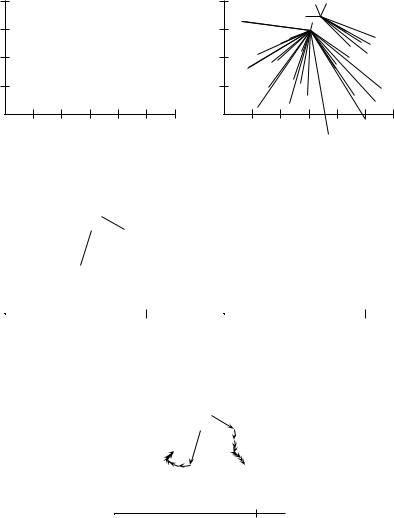
Figure 16.7 The outcome of clustering in K-means depends on the initial seeds. For seeds d2 and d5, K-means converges to {{d1, d2, d3}, {d4, d5, d6}}, a suboptimal clustering. For seeds d2 and d3, it converges to {{d1, d2, d4, d5}, {d3, d6}}, the global optimum for K = 2.
Another type of suboptimal clustering that frequently occurs is one with empty clusters (Exercise 16.11).
Effective heuristics for seed selection include (i) excluding outliers from the seed set; (ii) trying out multiple starting points and choosing the clustering with lowest cost; and (iii) obtaining seeds from another method such as hierarchical clustering. Since deterministic hierarchical clustering methods are more predictable than K-means, a hierarchical clustering of a small random sample of size iK (e.g., for i = 5 or i = 10) often provides good seeds (see the description of the Buckshot algorithm, Chapter 17, page 399).
Other initialization methods compute seeds that are not selected from the vectors to be clustered. A robust method that works well for a large variety of document distributions is to select i (e.g., i = 10) random vectors for each cluster and use their centroid as the seed for this cluster. See Section 16.6 for more sophisticated initializations.
What is the time complexity of K-means? Most of the time is spent on computing vector distances. One such operation costs Θ(M). The reassignment step computes KN distances, so its overall complexity is Θ(KN M). In the recomputation step, each vector gets added to a centroid once, so the complexity of this step is Θ(N M). For a fixed number of iterations I, the overall complexity is therefore Θ(IKN M). Thus, K-means is linear in all relevant factors: iterations, number of clusters, number of vectors and dimensionality of the space. This means that K-means is more efficient than the hierarchical algorithms in Chapter 17. We had to fix the number of iterations I, which can be tricky in practice. But in most cases, K-means quickly reaches either complete convergence or a clustering that is close to convergence. In the latter case, a few documents would switch membership if further iterations were computed, but this has a small effect on the overall quality of the clustering.
Online edition (c) 2009 Cambridge UP