4.3 Single-pass in-memory indexing

SPIMI-INVERT(token_stream)

1output_ f ile = NEWFILE()

2dictionary = NEWHASH()

3 while (free memory available) 4 do token ← next(token_stream)

5if term(token) / dictionary

6 then postings_list = ADDTODICTIONARY(dictionary, term(token)) 7 else postings_list = GETPOSTINGSLIST(dictionary, term(token))

8if f ull( postings_list)

9then postings_list = DOUBLEPOSTINGSLIST(dictionary, term(token))

10ADDTOPOSTINGSLIST( postings_list, docID(token))

11sorted_terms ← SORTTERMS(dictionary)

12WRITEBLOCKTODISK(sorted_terms, dictionary, output_ f ile)

13return output_ f ile

Figure 4.4 Inversion of a block in single-pass in-memory indexing

4.3Single-pass in-memory indexing

Online edition (c) 2009 Cambridge UP

list belongs to, so the termIDs of postings need not be stored. As a result, the blocks that individual calls of SPIMI-INVERT can process are much larger and the index construction process as a whole is more efficient.

Because we do not know how large the postings list of a term will be when we first encounter it, we allocate space for a short postings list initially and double the space each time it is full (lines 8–9). This means that some memory is wasted, which counteracts the memory savings from the omission of termIDs in intermediate data structures. However, the overall memory requirements for the dynamically constructed index of a block in SPIMI are still lower than in BSBI.

When memory has been exhausted, we write the index of the block (which consists of the dictionary and the postings lists) to disk (line 12). We have to sort the terms (line 11) before doing this because we want to write postings lists in lexicographic order to facilitate the final merging step. If each block’s postings lists were written in unsorted order, merging blocks could not be accomplished by a simple linear scan through each block.

Each call of SPIMI-INVERT writes a block to disk, just as in BSBI. The last step of SPIMI (corresponding to line 7 in Figure 4.2; not shown in Figure 4.4) is then to merge the blocks into the final inverted index.

In addition to constructing a new dictionary structure for each block and eliminating the expensive sorting step, SPIMI has a third important component: compression. Both the postings and the dictionary terms can be stored compactly on disk if we employ compression. Compression increases the efficiency of the algorithm further because we can process even larger blocks, and because the individual blocks require less space on disk. We refer readers to the literature for this aspect of the algorithm (Section 4.7).

The time complexity of SPIMI is Θ(T) because no sorting of tokens is required and all operations are at most linear in the size of the collection.

4.4Distributed indexing

Collections are often so large that we cannot perform index construction efficiently on a single machine. This is particularly true of the World Wide Web for which we need large computer clusters1 to construct any reasonably sized web index. Web search engines, therefore, use distributed indexing algorithms for index construction. The result of the construction process is a distributed index that is partitioned across several machines – either according to term or according to document. In this section, we describe distributed indexing for a term-partitioned index. Most large search engines prefer a document-

1. A cluster in this chapter is a group of tightly coupled computers that work together closely. This sense of the word is different from the use of cluster as a group of documents that are semantically similar in Chapters 16–18.

Online edition (c) 2009 Cambridge UP

Online edition (c) 2009 Cambridge UP

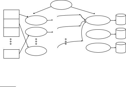
Figure 4.5 An example of distributed indexing with MapReduce. Adapted from Dean and Ghemawat (2004).

partitioning the keys into j term partitions and having the parsers write keyvalue pairs for each term partition into a separate segment file. In Figure 4.5, the term partitions are according to first letter: a–f, g–p, q–z, and j = 3. (We chose these key ranges for ease of exposition. In general, key ranges need not correspond to contiguous terms or termIDs.) The term partitions are defined by the person who operates the indexing system (Exercise 4.10). The parsers then write corresponding segment files, one for each term partition. Each term partition thus corresponds to r segments files, where r is the number of parsers. For instance, Figure 4.5 shows three a–f segment files of the a–f partition, corresponding to the three parsers shown in the figure.

Collecting all values (here: docIDs) for a given key (here: termID) into one INVERTER list is the task of the inverters in the reduce phase. The master assigns each term partition to a different inverter – and, as in the case of parsers, reassigns term partitions in case of failing or slow inverters. Each term partition (corresponding to r segment files, one on each parser) is processed by one inverter. We assume here that segment files are of a size that a single machine can handle (Exercise 4.9). Finally, the list of values is sorted for each key and written to the final sorted postings list (“postings” in the figure). (Note that postings in Figure 4.6 include term frequencies, whereas each posting in the other sections of this chapter is simply a docID without term frequency information.) The data flow is shown for a–f in Figure 4.5. This completes the

construction of the inverted index.

Online edition (c) 2009 Cambridge UP

Figure 4.6 Map and reduce functions in MapReduce. In general, the map function produces a list of key-value pairs. All values for a key are collected into one list in the reduce phase. This list is then processed further. The instantiations of the two functions and an example are shown for index construction. Because the map phase processes documents in a distributed fashion, termID–docID pairs need not be ordered correctly initially as in this example. The example shows terms instead of termIDs for better readability. We abbreviate Caesar as C and conquered as c'ed.

Parsers and inverters are not separate sets of machines. The master identifies idle machines and assigns tasks to them. The same machine can be a parser in the map phase and an inverter in the reduce phase. And there are often other jobs that run in parallel with index construction, so in between being a parser and an inverter a machine might do some crawling or another unrelated task.

To minimize write times before inverters reduce the data, each parser writes its segment files to its local disk. In the reduce phase, the master communicates to an inverter the locations of the relevant segment files (e.g., of the r segment files of the a–f partition). Each segment file only requires one sequential read because all data relevant to a particular inverter were written to a single segment file by the parser. This setup minimizes the amount of network traffic needed during indexing.

Figure 4.6 shows the general schema of the MapReduce functions. Input and output are often lists of key-value pairs themselves, so that several MapReduce jobs can run in sequence. In fact, this was the design of the Google indexing system in 2004. What we describe in this section corresponds to only one of five to ten MapReduce operations in that indexing system. Another MapReduce operation transforms the term-partitioned index we just created into a document-partitioned one.

MapReduce offers a robust and conceptually simple framework for implementing index construction in a distributed environment. By providing a semiautomatic method for splitting index construction into smaller tasks, it can scale to almost arbitrarily large collections, given computer clusters of

Online edition (c) 2009 Cambridge UP