

- •List of Tables
- •List of Figures
- •Table of Notation
- •Preface
- •Boolean retrieval
- •An example information retrieval problem
- •Processing Boolean queries
- •The extended Boolean model versus ranked retrieval
- •References and further reading
- •The term vocabulary and postings lists
- •Document delineation and character sequence decoding
- •Obtaining the character sequence in a document
- •Choosing a document unit
- •Determining the vocabulary of terms
- •Tokenization
- •Dropping common terms: stop words
- •Normalization (equivalence classing of terms)
- •Stemming and lemmatization
- •Faster postings list intersection via skip pointers
- •Positional postings and phrase queries
- •Biword indexes
- •Positional indexes
- •Combination schemes
- •References and further reading
- •Dictionaries and tolerant retrieval
- •Search structures for dictionaries
- •Wildcard queries
- •General wildcard queries
- •Spelling correction
- •Implementing spelling correction
- •Forms of spelling correction
- •Edit distance
- •Context sensitive spelling correction
- •Phonetic correction
- •References and further reading
- •Index construction
- •Hardware basics
- •Blocked sort-based indexing
- •Single-pass in-memory indexing
- •Distributed indexing
- •Dynamic indexing
- •Other types of indexes
- •References and further reading
- •Index compression
- •Statistical properties of terms in information retrieval
- •Dictionary compression
- •Dictionary as a string
- •Blocked storage
- •Variable byte codes
- •References and further reading
- •Scoring, term weighting and the vector space model
- •Parametric and zone indexes
- •Weighted zone scoring
- •Learning weights
- •The optimal weight g
- •Term frequency and weighting
- •Inverse document frequency
- •The vector space model for scoring
- •Dot products
- •Queries as vectors
- •Computing vector scores
- •Sublinear tf scaling
- •Maximum tf normalization
- •Document and query weighting schemes
- •Pivoted normalized document length
- •References and further reading
- •Computing scores in a complete search system
- •Index elimination
- •Champion lists
- •Static quality scores and ordering
- •Impact ordering
- •Cluster pruning
- •Components of an information retrieval system
- •Tiered indexes
- •Designing parsing and scoring functions
- •Putting it all together
- •Vector space scoring and query operator interaction
- •References and further reading
- •Evaluation in information retrieval
- •Information retrieval system evaluation
- •Standard test collections
- •Evaluation of unranked retrieval sets
- •Evaluation of ranked retrieval results
- •Assessing relevance
- •A broader perspective: System quality and user utility
- •System issues
- •User utility
- •Results snippets
- •References and further reading
- •Relevance feedback and query expansion
- •Relevance feedback and pseudo relevance feedback
- •The Rocchio algorithm for relevance feedback
- •Probabilistic relevance feedback
- •When does relevance feedback work?
- •Relevance feedback on the web
- •Evaluation of relevance feedback strategies
- •Pseudo relevance feedback
- •Indirect relevance feedback
- •Summary
- •Global methods for query reformulation
- •Vocabulary tools for query reformulation
- •Query expansion
- •Automatic thesaurus generation
- •References and further reading
- •XML retrieval
- •Basic XML concepts
- •Challenges in XML retrieval
- •A vector space model for XML retrieval
- •Evaluation of XML retrieval
- •References and further reading
- •Exercises
- •Probabilistic information retrieval
- •Review of basic probability theory
- •The Probability Ranking Principle
- •The 1/0 loss case
- •The PRP with retrieval costs
- •The Binary Independence Model
- •Deriving a ranking function for query terms
- •Probability estimates in theory
- •Probability estimates in practice
- •Probabilistic approaches to relevance feedback
- •An appraisal and some extensions
- •An appraisal of probabilistic models
- •Bayesian network approaches to IR
- •References and further reading
- •Language models for information retrieval
- •Language models
- •Finite automata and language models
- •Types of language models
- •Multinomial distributions over words
- •The query likelihood model
- •Using query likelihood language models in IR
- •Estimating the query generation probability
- •Language modeling versus other approaches in IR
- •Extended language modeling approaches
- •References and further reading
- •Relation to multinomial unigram language model
- •The Bernoulli model
- •Properties of Naive Bayes
- •A variant of the multinomial model
- •Feature selection
- •Mutual information
- •Comparison of feature selection methods
- •References and further reading
- •Document representations and measures of relatedness in vector spaces
- •k nearest neighbor
- •Time complexity and optimality of kNN
- •The bias-variance tradeoff
- •References and further reading
- •Exercises
- •Support vector machines and machine learning on documents
- •Support vector machines: The linearly separable case
- •Extensions to the SVM model
- •Multiclass SVMs
- •Nonlinear SVMs
- •Experimental results
- •Machine learning methods in ad hoc information retrieval
- •Result ranking by machine learning
- •References and further reading
- •Flat clustering
- •Clustering in information retrieval
- •Problem statement
- •Evaluation of clustering
- •Cluster cardinality in K-means
- •Model-based clustering
- •References and further reading
- •Exercises
- •Hierarchical clustering
- •Hierarchical agglomerative clustering
- •Time complexity of HAC
- •Group-average agglomerative clustering
- •Centroid clustering
- •Optimality of HAC
- •Divisive clustering
- •Cluster labeling
- •Implementation notes
- •References and further reading
- •Exercises
- •Matrix decompositions and latent semantic indexing
- •Linear algebra review
- •Matrix decompositions
- •Term-document matrices and singular value decompositions
- •Low-rank approximations
- •Latent semantic indexing
- •References and further reading
- •Web search basics
- •Background and history
- •Web characteristics
- •The web graph
- •Spam
- •Advertising as the economic model
- •The search user experience
- •User query needs
- •Index size and estimation
- •Near-duplicates and shingling
- •References and further reading
- •Web crawling and indexes
- •Overview
- •Crawling
- •Crawler architecture
- •DNS resolution
- •The URL frontier
- •Distributing indexes
- •Connectivity servers
- •References and further reading
- •Link analysis
- •The Web as a graph
- •Anchor text and the web graph
- •PageRank
- •Markov chains
- •The PageRank computation
- •Hubs and Authorities
- •Choosing the subset of the Web
- •References and further reading
- •Bibliography
- •Author Index
19.6 Near-duplicates and shingling |
437 |
2.Picking from the top 100 results of E1 induces a bias from the ranking algorithm of E1. Picking from all the results of E1 makes the experiment slower. This is particularly so because most web search engines put up defenses against excessive robotic querying.
3.During the checking phase, a number of additional biases are introduced: for instance, E2 may not handle 8-word conjunctive queries properly.
4.Either E1 or E2 may refuse to respond to the test queries, treating them as robotic spam rather than as bona fide queries.
5.There could be operational problems like connection time-outs.
A sequence of research has built on this basic paradigm to eliminate some of these issues; there is no perfect solution yet, but the level of sophistication in statistics for understanding the biases is increasing. The main idea is to address biases by estimating, for each document, the magnitude of the bias. From this, standard statistical sampling methods can generate unbiased samples. In the checking phase, the newer work moves away from conjunctive queries to phrase and other queries that appear to be betterbehaved. Finally, newer experiments use other sampling methods besides random queries. The best known of these is document random walk sampling, in which a document is chosen by a random walk on a virtual graph derived from documents. In this graph, nodes are documents; two documents are connected by an edge if they share two or more words in common. The graph is never instantiated; rather, a random walk on it can be performed by moving from a document d to another by picking a pair of keywords in d, running a query on a search engine and picking a random document from the results. Details may be found in the references in Section 19.7.
?Exercise 19.7
Two web search engines A and B each generate a large number of pages uniformly at random from their indexes. 30% of A’s pages are present in B’s index, while 50% of B’s pages are present in A’s index. What is the number of pages in A’s index relative to B’s?
19.6Near-duplicates and shingling
One aspect we have ignored in the discussion of index size in Section 19.5 is duplication: the Web contains multiple copies of the same content. By some estimates, as many as 40% of the pages on the Web are duplicates of other pages. Many of these are legitimate copies; for instance, certain information repositories are mirrored simply to provide redundancy and access reliability. Search engines try to avoid indexing multiple copies of the same content, to keep down storage and processing overheads.
Online edition (c) 2009 Cambridge UP
438 |
19 Web search basics |
The simplest approach to detecting duplicates is to compute, for each web page, a fingerprint that is a succinct (say 64-bit) digest of the characters on that page. Then, whenever the fingerprints of two web pages are equal, we test whether the pages themselves are equal and if so declare one of them to be a duplicate copy of the other. This simplistic approach fails to capture a crucial and widespread phenomenon on the Web: near duplication. In many cases, the contents of one web page are identical to those of another except for a few characters – say, a notation showing the date and time at which the page was last modified. Even in such cases, we want to be able to declare the two pages to be close enough that we only index one copy. Short of exhaustively comparing all pairs of web pages, an infeasible task at the scale of billions of pages, how can we detect and filter out such near duplicates?
We now describe a solution to the problem of detecting near-duplicate web SHINGLING pages. The answer lies in a technique known as shingling. Given a positive integer k and a sequence of terms in a document d, define the k-shingles of d to be the set of all consecutive sequences of k terms in d. As an example, consider the following text: a rose is a rose is a rose. The 4-shingles for this text (k = 4 is a typical value used in the detection of near-duplicate web pages) are a rose is a, rose is a rose and is a rose is. The first two of these shingles each occur twice in the text. Intuitively, two documents are near duplicates if the sets of shingles generated from them are nearly the same. We now make this intuition precise, then develop a method for efficiently computing and
comparing the sets of shingles for all web pages.
Let S(dj) denote the set of shingles of document dj. Recall the Jaccard coefficient from page 61, which measures the degree of overlap between
the sets S(d1) and S(d2) as |S(d1) ∩ S(d2)|/|S(d1) S(d2)|; denote this by J(S(d1), S(d2)). Our test for near duplication between d1 and d2 is to com-
pute this Jaccard coefficient; if it exceeds a preset threshold (say, 0.9), we declare them near duplicates and eliminate one from indexing. However, this does not appear to have simplified matters: we still have to compute Jaccard coefficients pairwise.
To avoid this, we use a form of hashing. First, we map every shingle into a hash value over a large space, say 64 bits. For j = 1, 2, let H(dj) be the corresponding set of 64-bit hash values derived from S(dj). We now invoke the following trick to detect document pairs whose sets H() have large Jaccard overlaps. Let π be a random permutation from the 64-bit integers to the 64-bit integers. Denote by Π(dj) the set of permuted hash values in H(dj); thus for each h H(dj), there is a corresponding value π(h) Π(dj).
Let xπj be the smallest integer in Π(dj). Then
Theorem 19.1.
J(S(d1), S(d2)) = P(x1π = x2π ).
Online edition (c) 2009 Cambridge UP
19.6 |
Near-duplicates and shingling |
|
|
|
|
|
|
439 |
|
|
||||||
|
|
|
H(d1) |
|
|
|
|
|
|
|
|
H(d2) |
|
|
|
|
0 |
|
u u |
u u |
- |
264 |
− |
1 |
|
0 |
u |
u u u |
- |
264 |
− |
1 |
|
|
|
1 2 |
3 4 |
|
|
|
|
|
1 |
2 3 4 |
|
|
|
|||
|
|
H(d1) and Π(d1) |
|
|
|
|
|
|
H(d2) and Π(d2) |
|
|
|
|
|||
0 |
3 |
u u 1 4 u u 2 |
- |
264 − 1 |
|
0 |
3 u |
1 u 4 u u |
2- |
264 − 1 |
||||||
|
|
|
Π(d1) |
|
|
|
|
|
|
|
|
Π(d2) |
|
|
|
|
0 |
3 |
1 4 |
2 |
- |
264 − 1 |
|
0 |
3 |
1 4 |
2- |
264 − 1 |
|||||
|
x1π |
|
|
|
- |
264 − 1 |
|
|
x2π |
|
- |
264 − 1 |
||||
0 |
3 |
|
|
|
|
0 |
3 |
|
||||||||
|
Document 1 |
|
|
|
|
|
|
|
Document 2 |
|
|
|
|
|||
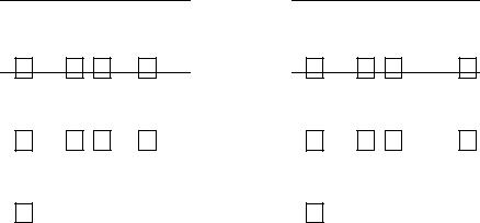
Figure 19.8 Illustration of shingle sketches. We see two documents going through |
|
|
||||||||||||||
four stages of shingle sketch computation. In the first step (top row), we apply a 64-bit |
|
|
||||||||||||||
hash to each shingle from each document to obtain H(d1) and H(d2) (circles). Next, |
|
|
||||||||||||||
we apply a random permutation Π to permute H(d1) and H(d2), obtaining Π(d1) |
|
|
||||||||||||||
and Π(d2) (squares). The third row shows only Π(d1) and Π(d2), while the bottom |
|
|
||||||||||||||
row shows the minimum values xπ and xπ for each document. |
|
|
|
|
||||||||||||
|
|
|
|
|
1 |
|
|
2 |
|
|
|
|
|
|
|
|
Proof. We give the proof in a slightly more general setting: consider a family of sets whose elements are drawn from a common universe. View the sets as columns of a matrix A, with one row for each element in the universe. The element aij = 1 if element i is present in the set Sj that the jth column represents.
Let Π be a random permutation of the rows of A; denote by Π(Sj) the column that results from applying Π to the jth column. Finally, let xπj be the
index of the first row in which the column Π(Sj) has a 1. We then prove that for any two columns j1, j2,
P(xπj1 = xπj2 ) = J(Sj1 , Sj2 ).
If we can prove this, the theorem follows.
Consider two columns j1, j2 as shown in Figure 19.9. The ordered pairs of entries of Sj1 and Sj2 partition the rows into four types: those with 0’s in both of these columns, those with a 0 in Sj1 and a 1 in Sj2 , those with a 1 in Sj1 and a 0 in Sj2 , and finally those with 1’s in both of these columns. Indeed, the first four rows of Figure 19.9 exemplify all of these four types of rows.
Online edition (c) 2009 Cambridge UP

440 |
|
|
19 Web search basics |
|
|
|
|
|
Sj |
Sj |
|
|
1 |
2 |
|
|
0 |
1 |
|
|
1 |
0 |
|
|
1 |
1 |
|
|
0 |
0 |
|
|
1 |
1 |
|
|
0 |
1 |
|
Figure 19.9 Two sets Sj1 and Sj2 ; their Jaccard coefficient is 2/5.
Denote by C00 the number of rows with 0’s in both columns, C01 the second, C10 the third and C11 the fourth. Then,
(19.2) |
J(Sj |
, Sj ) = |
|
C11 |
. |
|
|
||||
|
1 |
2 |
C01 |
+ C10 + C11 |
|
|
|
|
|
||
To complete the proof by showing that the right-hand side of Equation (19.2) |
|||||
equals P(xπ |
= xπ ), consider scanning columns j , j in increasing row in- |
||||
j1 |
j2 |
|
|
1 |
2 |
dex until the first non-zero entry is found in either column. Because Π is a random permutation, the probability that this smallest row has a 1 in both columns is exactly the right-hand side of Equation (19.2). 
Thus, our test for the Jaccard coefficient of the shingle sets is probabilistic: we compare the computed values xiπ from different documents. If a pair coincides, we have candidate near duplicates. Repeat the process independently for 200 random permutations π (a choice suggested in the literature). Call the set of the 200 resulting values of xiπ the sketch ψ(di) of di. We can then estimate the Jaccard coefficient for any pair of documents di, dj to be |ψi ∩ ψj|/200; if this exceeds a preset threshold, we declare that di and dj are similar.
How can we quickly compute |ψi ∩ ψj|/200 for all pairs i, j? Indeed, how do we represent all pairs of documents that are similar, without incurring a blowup that is quadratic in the number of documents? First, we use fingerprints to remove all but one copy of identical documents. We may also remove common HTML tags and integers from the shingle computation, to eliminate shingles that occur very commonly in documents without telling us anything about duplication. Next we use a union-find algorithm to create clusters that contain documents that are similar. To do this, we must accomplish a crucial step: going from the set of sketches to the set of pairs i, j such that di and dj are similar.
To this end, we compute the number of shingles in common for any pair of documents whose sketches have any members in common. We begin with the list < xiπ , di > sorted by xiπ pairs. For each xiπ , we can now generate
Online edition (c) 2009 Cambridge UP