SELECTFEATURES(D, c, k)

1 V ← EXTRACTVOCABULARY(D)

2L ← []

3for each t V

4do A(t, c) ← COMPUTEFEATUREUTILITY(D, t, c)

5APPEND(L, hA(t, c), ti)

6return FEATURESWITHLARGESTVALUES(L, k)

Figure 13.6 Basic feature selection algorithm for selecting the k best features.

ences, describe them.

Exercise 13.3

The rationale for the positional independence assumption is that there is no useful information in the fact that a term occurs in position k of a document. Find exceptions. Consider formulaic documents with a fixed document structure.

Exercise 13.4

Table 13.3 gives Bernoulli and multinomial estimates for the word the. Explain the difference.

13.5Feature selection

Online edition (c) 2009 Cambridge UP

It may appear counterintuitive at first that a seemingly weaker classifier is advantageous in statistical text classification, but when discussing the biasvariance tradeoff in Section 14.6 (page 308), we will see that weaker models are often preferable when limited training data are available.

The basic feature selection algorithm is shown in Figure 13.6. For a given class c, we compute a utility measure A(t, c) for each term of the vocabulary and select the k terms that have the highest values of A(t, c). All other terms are discarded and not used in classification. We will introduce three different

utility measures in this section: mutual information, A(t, c) = I(Ut; Cc); the χ2 test, A(t, c) = X2(t, c); and frequency, A(t, c) = N(t, c).

Of the two NB models, the Bernoulli model is particularly sensitive to noise features. A Bernoulli NB classifier requires some form of feature selection or else its accuracy will be low.

This section mainly addresses feature selection for two-class classification tasks like China versus not-China. Section 13.5.5 briefly discusses optimizations for systems with more than two classes.

13.5.1Mutual information

A common feature selection method is to compute A(t, c) as the expected MUTUAL INFORMATION mutual information (MI) of term t and class c.5 MI measures how much information the presence/absence of a term contributes to making the correct

classification decision on c. Formally:

where the Ns are counts of documents that have the values of et and ec that are indicated by the two subscripts. For example, N10 is the number of doc-

5. Take care not to confuse expected mutual information with pointwise mutual information, which is defined as log N11/E11 where N11 and E11 are defined as in Equation (13.18). The two measures have different properties. See Section 13.7.

Online edition (c) 2009 Cambridge UP

the number of documents that contain t (et = 1) and we count documents

independent of class membership (ec {0, 1}). N = N00 + N01 + N10 + N11 is the total number of documents. An example of one of the MLE estimates

that transform Equation (13.16) into Equation (13.17) is P(U = 1, C = 1) =

N11/N.

Example 13.3: Consider the class poultry and the term export in Reuters-RCV1. The counts of the number of documents with the four possible combinations of indicator values are as follows:

After plugging these values into Equation (13.17) we get:

141801,948 · 141

+801,948 log2 (141+774,106)(49+141)

+ 774,106801,948 log2 (141+774,106)(27,652+774,106)

≈0.0001105 801,948 · 774,106

To select k terms t1, . . . , tk for a given class, we use the feature selection algorithm in Figure 13.6: We compute the utility measure as A(t, c) = I(Ut, Cc) and select the k terms with the largest values.

Mutual information measures how much information – in the informationtheoretic sense – a term contains about the class. If a term’s distribution is the same in the class as it is in the collection as a whole, then I(U; C) = 0. MI reaches its maximum value if the term is a perfect indicator for class membership, that is, if the term is present in a document if and only if the document is in the class.

Figure 13.7 shows terms with high mutual information scores for the six classes in Figure 13.1.6 The selected terms (e.g., london, uk, british for the class UK) are of obvious utility for making classification decisions for their respective classes. At the bottom of the list for UK we find terms like peripherals and tonight (not shown in the figure) that are clearly not helpful in deciding

6. Feature scores were computed on the first 100,000 documents, except for poultry, a rare class, for which 800,000 documents were used. We have omitted numbers and other special words from the top ten lists.

Online edition (c) 2009 Cambridge UP

Figure 13.7 Features with high mutual information scores for six Reuters-RCV1 classes.

whether the document is in the class. As you might expect, keeping the informative terms and eliminating the non-informative ones tends to reduce noise and improve the classifier’s accuracy.

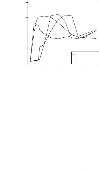
Such an accuracy increase can be observed in Figure 13.8, which shows F1 as a function of vocabulary size after feature selection for Reuters-RCV1.7 Comparing F1 at 132,776 features (corresponding to selection of all features) and at 10–100 features, we see that MI feature selection increases F1 by about 0.1 for the multinomial model and by more than 0.2 for the Bernoulli model. For the Bernoulli model, F1 peaks early, at ten features selected. At that point, the Bernoulli model is better than the multinomial model. When basing a classification decision on only a few features, it is more robust to consider binary occurrence only. For the multinomial model (MI feature selection), the peak occurs later, at 100 features, and its effectiveness recovers somewhat at

7. We trained the classifiers on the first 100,000 documents and computed F1 on the next 100,000. The graphs are averages over five classes.

Online edition (c) 2009 Cambridge UP

number of features selected

Figure 13.8 Effect of feature set size on accuracy for multinomial and Bernoulli models.

the end when we use all features. The reason is that the multinomial takes the number of occurrences into account in parameter estimation and classification and therefore better exploits a larger number of features than the Bernoulli model. Regardless of the differences between the two methods, using a carefully selected subset of the features results in better effectiveness than using all features.

13.5.2χ2 Feature selection

Online edition (c) 2009 Cambridge UP

Online edition (c) 2009 Cambridge UP

Critical values of the χ2 distribution with one degree of freedom. For example, if the two events are independent, then P(X2 > 6.63) < 0.01. So for X2 > 6.63 the assumption of independence can be rejected with 99% confidence.

pχ2 critical value

0.12.71

0.053.84

0.01 6.63

0.005 7.88

0.001 10.83

χ

test with one degree of freedom, the so-called Yates correction should be used (see Section 13.7), which makes it harder to reach statistical significance. Also, whenever a statistical test is used multiple times, then the probability of getting at least one error increases. If 1,000 hypotheses are rejected, each with 0.05 error probability, then 0.05 × 1000 = 50 calls of the test will be wrong on average. However, in text classification it rarely matters whether a few additional terms are added to the feature set or removed from it. Rather, the relative importance of features is important. As long as χ2 feature selection only ranks features with respect to their usefulness and is not used to make statements about statistical dependence or independence of variables, we need not be overly concerned that it does not adhere strictly to statistical theory.

13.5.3Frequency-based feature selection

A third feature selection method is frequency-based feature selection, that is, selecting the terms that are most common in the class. Frequency can be either defined as document frequency (the number of documents in the class c that contain the term t) or as collection frequency (the number of tokens of t that occur in documents in c). Document frequency is more appropriate for the Bernoulli model, collection frequency for the multinomial model.

Frequency-based feature selection selects some frequent terms that have no specific information about the class, for example, the days of the week (Monday, Tuesday, . . . ), which are frequent across classes in newswire text. When many thousands of features are selected, then frequency-based feature selection often does well. Thus, if somewhat suboptimal accuracy is acceptable, then frequency-based feature selection can be a good alternative to more complex methods. However, Figure 13.8 is a case where frequency-

Online edition (c) 2009 Cambridge UP