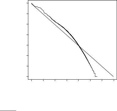
Figure 5.2 Zipf’s law for Reuters-RCV1. Frequency is plotted as a function of frequency rank for the terms in the collection. The line is the distribution predicted by Zipf’s law (weighted least-squares fit; intercept is 6.95).

5.2 Dictionary compression

This section presents a series of dictionary data structures that achieve increasingly higher compression ratios. The dictionary is small compared with the postings file as suggested by Table 5.1. So why compress it if it is responsible for only a small percentage of the overall space requirements of the IR system?

One of the primary factors in determining the response time of an IR system is the number of disk seeks necessary to process a query. If parts of the dictionary are on disk, then many more disk seeks are necessary in query evaluation. Thus, the main goal of compressing the dictionary is to fit it in main memory, or at least a large portion of it, to support high query through-

Online edition (c) 2009 Cambridge UP

Figure 5.3 Storing the dictionary as an array of fixed-width entries.

put. Although dictionaries of very large collections fit into the memory of a standard desktop machine, this is not true of many other application scenarios. For example, an enterprise search server for a large corporation may have to index a multiterabyte collection with a comparatively large vocabulary because of the presence of documents in many different languages. We also want to be able to design search systems for limited hardware such as mobile phones and onboard computers. Other reasons for wanting to conserve memory are fast startup time and having to share resources with other applications. The search system on your PC must get along with the memory-hogging word processing suite you are using at the same time.

5.2.1Dictionary as a string

The simplest data structure for the dictionary is to sort the vocabulary lexicographically and store it in an array of fixed-width entries as shown in Figure 5.3. We allocate 20 bytes for the term itself (because few terms have more than twenty characters in English), 4 bytes for its document frequency, and 4 bytes for the pointer to its postings list. Four-byte pointers resolve a 4 gigabytes (GB) address space. For large collections like the web, we need to allocate more bytes per pointer. We look up terms in the array by binary search. For Reuters-RCV1, we need M × (20 + 4 + 4) = 400,000 × 28 = 11.2megabytes (MB) for storing the dictionary in this scheme.

Using fixed-width entries for terms is clearly wasteful. The average length of a term in English is about eight characters (Table 4.2, page 70), so on average we are wasting twelve characters in the fixed-width scheme. Also, we have no way of storing terms with more than twenty characters like hydrochlorofluorocarbons and supercalifragilisticexpialidocious. We can overcome these shortcomings by storing the dictionary terms as one long string of characters, as shown in Figure 5.4. The pointer to the next term is also used to demarcate the end of the current term. As before, we locate terms in the data structure by way of binary search in the (now smaller) table. This scheme saves us 60% compared to fixed-width storage – 12 bytes on average of the

Online edition (c) 2009 Cambridge UP

92 5 Index compression

. . . s y s t i l e s y z y g e t i c s y z y g i a l s y z y g y s z a i b e l y i t e s z e c i n s z o n o . . .

Figure 5.4 Dictionary-as-a-string storage. Pointers mark the end of the preceding term and the beginning of the next. For example, the first three terms in this example

are systile, syzygetic, and syzygial.

20 bytes we allocated for terms before. However, we now also need to store term pointers. The term pointers resolve 400,000 × 8 = 3.2 × 106 positions, so they need to be log2 3.2 × 106 ≈ 22 bits or 3 bytes long.

In this new scheme, we need 400,000 × (4 + 4 + 3 + 8) = 7.6 MB for the Reuters-RCV1 dictionary: 4 bytes each for frequency and postings pointer, 3 bytes for the term pointer, and 8 bytes on average for the term. So we have reduced the space requirements by one third from 11.2 to 7.6 MB.

5.2.2Blocked storage

We can further compress the dictionary by grouping terms in the string into blocks of size k and keeping a term pointer only for the first term of each block (Figure 5.5). We store the length of the term in the string as an additional byte at the beginning of the term. We thus eliminate k − 1 term pointers, but need an additional k bytes for storing the length of each term. For k = 4, we save (k − 1) × 3 = 9 bytes for term pointers, but need an additional k = 4 bytes for term lengths. So the total space requirements for the dictionary of Reuters-RCV1 are reduced by 5 bytes per four-term block, or a total of 400,000 × 1/4 × 5 = 0.5 MB, bringing us down to 7.1 MB.

Online edition (c) 2009 Cambridge UP

. . . 7 s y s t i l e 9 s y z y g e t i c 8 s y z y g i a l 6 s y z y g y11 s z a i b e l y i t e 6 s z e c i n . . .

Figure 5.5 Blocked storage with four terms per block. The first block consists of systile, syzygetic, syzygial, and syzygy with lengths of seven, nine, eight, and six characters, respectively. Each term is preceded by a byte encoding its length that indicates how many bytes to skip to reach subsequent terms.

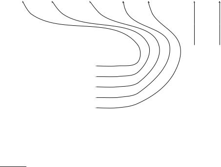
By increasing the block size k, we get better compression. However, there is a tradeoff between compression and the speed of term lookup. For the eight-term dictionary in Figure 5.6, steps in binary search are shown as double lines and steps in list search as simple lines. We search for terms in the uncompressed dictionary by binary search (a). In the compressed dictionary, we first locate the term’s block by binary search and then its position within the list by linear search through the block (b). Searching the uncompressed dictionary in (a) takes on average (0 + 1 + 2 + 3 + 2 + 1 + 2 + 2)/8 ≈ 1.6 steps, assuming each term is equally likely to come up in a query. For example, finding the two terms, aid and box, takes three and two steps, respectively. With blocks of size k = 4 in (b), we need (0 + 1 + 2 + 3 + 4 + 1 + 2 + 3)/8 = 2 steps on average, ≈ 25% more. For example, finding den takes one binary search step and two steps through the block. By increasing k, we can get the size of the compressed dictionary arbitrarily close to the minimum of 400,000 × (4 + 4 + 1 + 8) = 6.8 MB, but term lookup becomes prohibitively slow for large values of k.

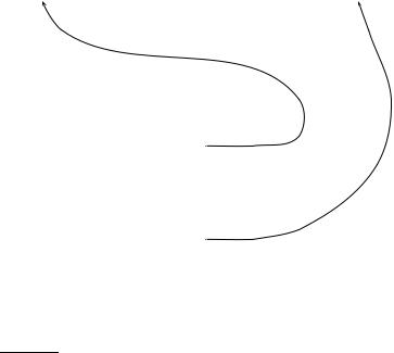
One source of redundancy in the dictionary we have not exploited yet is the fact that consecutive entries in an alphabetically sorted list share common FRONT CODING prefixes. This observation leads to front coding (Figure 5.7). A common prefix

Online edition (c) 2009 Cambridge UP

box

den

ex

job

ox

pit

win

(b)aid box den ex

job ox pit win

Figure 5.6 Search of the uncompressed dictionary (a) and a dictionary compressed by blocking with k = 4 (b).

One block in blocked compression (k = 4) . . .

8automata8automate9au t omatic10automation

. . . further compressed with front coding. 8automat a1 e2 ic3 i on

Figure 5.7 Front coding. A sequence of terms with identical prefix (“automat”) is encoded by marking the end of the prefix with and replacing it with in subsequent terms. As before, the first byte of each entry encodes the number of characters.

Online edition (c) 2009 Cambridge UP

Table 5.2 Dictionary compression for Reuters-RCV1.

is identified for a subsequence of the term list and then referred to with a special character. In the case of Reuters, front coding saves another 1.2 MB, as we found in an experiment.

Other schemes with even greater compression rely on minimal perfect hashing, that is, a hash function that maps M terms onto [1, . . . , M] without collisions. However, we cannot adapt perfect hashes incrementally because each new term causes a collision and therefore requires the creation of a new perfect hash function. Therefore, they cannot be used in a dynamic environment.

Even with the best compression scheme, it may not be feasible to store the entire dictionary in main memory for very large text collections and for hardware with limited memory. If we have to partition the dictionary onto pages that are stored on disk, then we can index the first term of each page using a B-tree. For processing most queries, the search system has to go to disk anyway to fetch the postings. One additional seek for retrieving the term’s dictionary page from disk is a significant, but tolerable increase in the time it takes to process a query.

Table 5.2 summarizes the compression achieved by the four dictionary data structures.

?Exercise 5.2

Estimate the space usage of the Reuters-RCV1 dictionary with blocks of size k = 8 and k = 16 in blocked dictionary storage.

Exercise 5.3

Estimate the time needed for term lookup in the compressed dictionary of ReutersRCV1 with block sizes of k = 4 (Figure 5.6, b), k = 8, and k = 16. What is the slowdown compared with k = 1 (Figure 5.6, a)?

5.3Postings file compression

Recall from Table 4.2 (page 70) that Reuters-RCV1 has 800,000 documents, 200 tokens per document, six characters per token, and 100,000,000 postings where we define a posting in this chapter as a docID in a postings list, that is, excluding frequency and position information. These numbers

Online edition (c) 2009 Cambridge UP