

- •List of Tables
- •List of Figures
- •Table of Notation
- •Preface
- •Boolean retrieval
- •An example information retrieval problem
- •Processing Boolean queries
- •The extended Boolean model versus ranked retrieval
- •References and further reading
- •The term vocabulary and postings lists
- •Document delineation and character sequence decoding
- •Obtaining the character sequence in a document
- •Choosing a document unit
- •Determining the vocabulary of terms
- •Tokenization
- •Dropping common terms: stop words
- •Normalization (equivalence classing of terms)
- •Stemming and lemmatization
- •Faster postings list intersection via skip pointers
- •Positional postings and phrase queries
- •Biword indexes
- •Positional indexes
- •Combination schemes
- •References and further reading
- •Dictionaries and tolerant retrieval
- •Search structures for dictionaries
- •Wildcard queries
- •General wildcard queries
- •Spelling correction
- •Implementing spelling correction
- •Forms of spelling correction
- •Edit distance
- •Context sensitive spelling correction
- •Phonetic correction
- •References and further reading
- •Index construction
- •Hardware basics
- •Blocked sort-based indexing
- •Single-pass in-memory indexing
- •Distributed indexing
- •Dynamic indexing
- •Other types of indexes
- •References and further reading
- •Index compression
- •Statistical properties of terms in information retrieval
- •Dictionary compression
- •Dictionary as a string
- •Blocked storage
- •Variable byte codes
- •References and further reading
- •Scoring, term weighting and the vector space model
- •Parametric and zone indexes
- •Weighted zone scoring
- •Learning weights
- •The optimal weight g
- •Term frequency and weighting
- •Inverse document frequency
- •The vector space model for scoring
- •Dot products
- •Queries as vectors
- •Computing vector scores
- •Sublinear tf scaling
- •Maximum tf normalization
- •Document and query weighting schemes
- •Pivoted normalized document length
- •References and further reading
- •Computing scores in a complete search system
- •Index elimination
- •Champion lists
- •Static quality scores and ordering
- •Impact ordering
- •Cluster pruning
- •Components of an information retrieval system
- •Tiered indexes
- •Designing parsing and scoring functions
- •Putting it all together
- •Vector space scoring and query operator interaction
- •References and further reading
- •Evaluation in information retrieval
- •Information retrieval system evaluation
- •Standard test collections
- •Evaluation of unranked retrieval sets
- •Evaluation of ranked retrieval results
- •Assessing relevance
- •A broader perspective: System quality and user utility
- •System issues
- •User utility
- •Results snippets
- •References and further reading
- •Relevance feedback and query expansion
- •Relevance feedback and pseudo relevance feedback
- •The Rocchio algorithm for relevance feedback
- •Probabilistic relevance feedback
- •When does relevance feedback work?
- •Relevance feedback on the web
- •Evaluation of relevance feedback strategies
- •Pseudo relevance feedback
- •Indirect relevance feedback
- •Summary
- •Global methods for query reformulation
- •Vocabulary tools for query reformulation
- •Query expansion
- •Automatic thesaurus generation
- •References and further reading
- •XML retrieval
- •Basic XML concepts
- •Challenges in XML retrieval
- •A vector space model for XML retrieval
- •Evaluation of XML retrieval
- •References and further reading
- •Exercises
- •Probabilistic information retrieval
- •Review of basic probability theory
- •The Probability Ranking Principle
- •The 1/0 loss case
- •The PRP with retrieval costs
- •The Binary Independence Model
- •Deriving a ranking function for query terms
- •Probability estimates in theory
- •Probability estimates in practice
- •Probabilistic approaches to relevance feedback
- •An appraisal and some extensions
- •An appraisal of probabilistic models
- •Bayesian network approaches to IR
- •References and further reading
- •Language models for information retrieval
- •Language models
- •Finite automata and language models
- •Types of language models
- •Multinomial distributions over words
- •The query likelihood model
- •Using query likelihood language models in IR
- •Estimating the query generation probability
- •Language modeling versus other approaches in IR
- •Extended language modeling approaches
- •References and further reading
- •Relation to multinomial unigram language model
- •The Bernoulli model
- •Properties of Naive Bayes
- •A variant of the multinomial model
- •Feature selection
- •Mutual information
- •Comparison of feature selection methods
- •References and further reading
- •Document representations and measures of relatedness in vector spaces
- •k nearest neighbor
- •Time complexity and optimality of kNN
- •The bias-variance tradeoff
- •References and further reading
- •Exercises
- •Support vector machines and machine learning on documents
- •Support vector machines: The linearly separable case
- •Extensions to the SVM model
- •Multiclass SVMs
- •Nonlinear SVMs
- •Experimental results
- •Machine learning methods in ad hoc information retrieval
- •Result ranking by machine learning
- •References and further reading
- •Flat clustering
- •Clustering in information retrieval
- •Problem statement
- •Evaluation of clustering
- •Cluster cardinality in K-means
- •Model-based clustering
- •References and further reading
- •Exercises
- •Hierarchical clustering
- •Hierarchical agglomerative clustering
- •Time complexity of HAC
- •Group-average agglomerative clustering
- •Centroid clustering
- •Optimality of HAC
- •Divisive clustering
- •Cluster labeling
- •Implementation notes
- •References and further reading
- •Exercises
- •Matrix decompositions and latent semantic indexing
- •Linear algebra review
- •Matrix decompositions
- •Term-document matrices and singular value decompositions
- •Low-rank approximations
- •Latent semantic indexing
- •References and further reading
- •Web search basics
- •Background and history
- •Web characteristics
- •The web graph
- •Spam
- •Advertising as the economic model
- •The search user experience
- •User query needs
- •Index size and estimation
- •Near-duplicates and shingling
- •References and further reading
- •Web crawling and indexes
- •Overview
- •Crawling
- •Crawler architecture
- •DNS resolution
- •The URL frontier
- •Distributing indexes
- •Connectivity servers
- •References and further reading
- •Link analysis
- •The Web as a graph
- •Anchor text and the web graph
- •PageRank
- •Markov chains
- •The PageRank computation
- •Hubs and Authorities
- •Choosing the subset of the Web
- •References and further reading
- •Bibliography
- •Author Index

13.4 Properties of Naive Bayes |
265 |
13.4Properties of Naive Bayes
To gain a better understanding of the two models and the assumptions they make, let us go back and examine how we derived their classification rules in Chapters 11 and 12. We decide class membership of a document by assigning it to the class with the maximum a posteriori probability (cf. Section 11.3.2, page 226), which we compute as follows:
cmap |
= |
arg max P(c|d) |
||
|
|
c C |
P(d|c)P(c) |
|
(13.9) |
= |
arg max |
|
|
|
|
c C |
P(d) |
|
|
|
|
|
|
(13.10) |
= |
arg max P(d|c)P(c), |
||
|
|
c C |
|
|
where Bayes’ rule (Equation (11.4), page 220) is applied in (13.9) and we drop the denominator in the last step because P(d) is the same for all classes and does not affect the argmax.
We can interpret Equation (13.10) as a description of the generative process we assume in Bayesian text classification. To generate a document, we first choose class c with probability P(c) (top nodes in Figures 13.4 and 13.5). The two models differ in the formalization of the second step, the generation of the document given the class, corresponding to the conditional distribution
P(d|c):
(13.11) |
Multinomial |
P(d|c) |
= |
P(ht1, . . . , tk, . . . , tnd i|c) |
(13.12) |
Bernoulli |
P(d|c) |
= |
P(he1, . . . , ei, . . . , eMi|c), |
where ht1, . . . , tnd i is the sequence of terms as it occurs in d (minus terms that were excluded from the vocabulary) and he1, . . . , ei, . . . , eMi is a binary vector of dimensionality M that indicates for each term whether it occurs in d or not.
It should now be clearer why we introduced the document space X in Equation (13.1) when we defined the classification problem. A critical step in solving a text classification problem is to choose the document representation. ht1, . . . , tnd i and he1, . . . , eMi are two different document representations. In the first case, X is the set of all term sequences (or, more precisely, sequences of term tokens). In the second case, X is {0, 1}M.
We cannot use Equations (13.11) and (13.12) for text classification directly. For the Bernoulli model, we would have to estimate 2M|C| different parameters, one for each possible combination of M values ei and a class. The number of parameters in the multinomial case has the same order of magni-
Online edition (c) 2009 Cambridge UP
266
CONDITIONAL
INDEPENDENCE
ASSUMPTION
(13.13)
(13.14)
RANDOM VARIABLE X
RANDOM VARIABLE U
13 Text classification and Naive Bayes
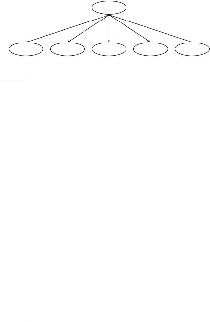
C=China
X1=Beijing |
X2=and |
X3=Taipei |
X4=join |
X5=WTO |
Figure 13.4 The multinomial NB model.
tude.3 This being a very large quantity, estimating these parameters reliably is infeasible.
To reduce the number of parameters, we make the Naive Bayes conditional independence assumption. We assume that attribute values are independent of each other given the class:
Multinomial |
P(d|c) |
= |
P(ht1, . . . , tnd i|c) = |
∏ P(Xk = tk|c) |
|
|
|
|
1≤k≤nd |
Bernoulli |
P(d|c) |
= |
P(he1, . . . , eMi|c) = |
∏ P(Ui = ei|c). |
|
|
|
|
1≤i≤M |
We have introduced two random variables here to make the two different generative models explicit. Xk is the random variable for position k in the document and takes as values terms from the vocabulary. P(Xk = t|c) is the probability that in a document of class c the term t will occur in position k. Ui is the random variable for vocabulary term i and takes as values 0 (absence)
and 1 (presence). ˆ( = 1| ) is the probability that in a document of class
P Ui c c the term ti will occur – in any position and possibly multiple times.
We illustrate the conditional independence assumption in Figures 13.4 and 13.5. The class China generates values for each of the five term attributes (multinomial) or six binary attributes (Bernoulli) with a certain probability, independent of the values of the other attributes. The fact that a document in the class China contains the term Taipei does not make it more likely or less likely that it also contains Beijing.
In reality, the conditional independence assumption does not hold for text data. Terms are conditionally dependent on each other. But as we will discuss shortly, NB models perform well despite the conditional independence assumption.
3. In fact, if the length of documents is not bounded, the number of parameters in the multinomial case is infinite.
Online edition (c) 2009 Cambridge UP

13.4 Properties of Naive Bayes |
267 |
C=China
UAlaska=0 |
UBeijing=1 |
UIndia=0 |
Ujoin=1 |
UTaipei=1 |
UWTO=1 |
Figure 13.5 The Bernoulli NB model.
POSITIONAL INDEPENDENCE
Even when assuming conditional independence, we still have too many parameters for the multinomial model if we assume a different probability distribution for each position k in the document. The position of a term in a document by itself does not carry information about the class. Although there is a difference between China sues France and France sues China, the occurrence of China in position 1 versus position 3 of the document is not useful in NB classification because we look at each term separately. The conditional independence assumption commits us to this way of processing the evidence.
Also, if we assumed different term distributions for each position k, we would have to estimate a different set of parameters for each k. The probability of bean appearing as the first term of a coffee document could be different from it appearing as the second term, and so on. This again causes problems in estimation owing to data sparseness.
For these reasons, we make a second independence assumption for the multinomial model, positional independence: The conditional probabilities for a term are the same independent of position in the document.
P(Xk1 = t|c) = P(Xk2 = t|c)
for all positions k1, k2, terms t and classes c. Thus, we have a single distribution of terms that is valid for all positions ki and we can use X as its symbol.4 Positional independence is equivalent to adopting the bag of words model, which we introduced in the context of ad hoc retrieval in Chapter 6 (page 117).
With conditional and positional independence assumptions, we only need
to estimate Θ(M|C|) parameters P(tk|c) (multinomial model) or P(ei|c) (Bernoulli
4. Our terminology is nonstandard. The random variable X is a categorical variable, not a multinomial variable, and the corresponding NB model should perhaps be called a sequence model. We have chosen to present this sequence model and the multinomial model in Section 13.4.1 as the same model because they are computationally identical.
Online edition (c) 2009 Cambridge UP
268 |
|
|
|
13 Text classification and Naive Bayes |
|
||
|
Table 13.3 Multinomial versus Bernoulli model. |
|
|
|
|||
|
|
|
multinomial model |
Bernoulli model |
|
||
|
event model |
generation of token |
generation of document |
||||
|
random variable(s) |
X = t iff t occurs at given pos |
Ut = 1 iff t occurs in doc |
||||
|
document representation |
d = ht1, . . . , tk, . . . , tnd i, tk V |
d = he1, . . . , ei, . . . , eMi, |
||||
|
parameter estimation |
ˆ |
|
ˆ ei {0, 1} |
|
||
|
P(X = t|c) |
ˆ |
P(Ui = e|c) |
|
|||
|
decision rule: maximize |
ˆ |
ˆ |
ˆ |
= ei|c) |
||
|
P(c) ∏1≤k≤nd |
P(X = tk|c) |
P(c) ∏ti V |
P(Ui |
|||
|
multiple occurrences |
taken into account |
ignored |
|
|
||
|
length of docs |
can handle longer docs |
works best for short docs |
||||
|
# features |
can handle more |
works best with fewer |
||||
|
estimate for term the |
ˆ |
|
ˆ |
|
1.0 |
|
|
P(X = the|c) ≈ 0.05 |
P(Uthe = 1|c) ≈ |
|||||
|
|
|
|
|
|
|
|
model), one for each term–class combination, rather than a number that is at least exponential in M, the size of the vocabulary. The independence assumptions reduce the number of parameters to be estimated by several orders of magnitude.
To summarize, we generate a document in the multinomial model (Fig- RANDOM VARIABLE C ure 13.4) by first picking a class C = c with P(c) where C is a random variable taking values from C as values. Next we generate term tk in position k with P(Xk = tk|c) for each of the nd positions of the document. The Xk all have the same distribution over terms for a given c. In the example in Figure 13.4, we show the generation of ht1, t2, t3, t4, t5i = hBeijing, and, Taipei, join, WTOi,
corresponding to the one-sentence document Beijing and Taipei join WTO. For a completely specified document generation model, we would also
have to define a distribution P(nd|c) over lengths. Without it, the multinomial model is a token generation model rather than a document generation model.
We generate a document in the Bernoulli model (Figure 13.5) by first picking a class C = c with P(c) and then generating a binary indicator ei for each term ti of the vocabulary (1 ≤ i ≤ M). In the example in Figure 13.5, we show the generation of he1, e2, e3, e4, e5, e6i = h0, 1, 0, 1, 1, 1i, corresponding, again, to the one-sentence document Beijing and Taipei join WTO where we have assumed that and is a stop word.
We compare the two models in Table 13.3, including estimation equations and decision rules.
Naive Bayes is so called because the independence assumptions we have just made are indeed very naive for a model of natural language. The conditional independence assumption states that features are independent of each other given the class. This is hardly ever true for terms in documents. In many cases, the opposite is true. The pairs hong and kong or london and en-
Online edition (c) 2009 Cambridge UP
13.4 Properties of Naive Bayes |
269 |
Table 13.4 Correct estimation implies accurate prediction, but accurate prediction does not imply correct estimation.
|
|
|
c1 |
c2 |
class selected |
|
true probability P(c|d) |
0.6 |
0.4 |
c1 |
|
|
ˆ |
ˆ |
|
0.00001 |
|
|
P(c) ∏1≤k≤nd ˆP(tk|c) (Equation (13.13)) 0.00099 |
|
|||
|
NB estimate P(c|d) |
0.99 |
0.01 |
c1 |
|
|
|
|
|
|
|
glish in Figure 13.7 are examples of highly dependent terms. In addition, the multinomial model makes an assumption of positional independence. The Bernoulli model ignores positions in documents altogether because it only cares about absence or presence. This bag-of-words model discards all information that is communicated by the order of words in natural language sentences. How can NB be a good text classifier when its model of natural language is so oversimplified?
The answer is that even though the probability estimates of NB are of low quality, its classification decisions are surprisingly good. Consider a document d with true probabilities P(c1|d) = 0.6 and P(c2|d) = 0.4 as shown in Table 13.4. Assume that d contains many terms that are positive indicators for
c1 and many terms that are negative indicators for c2. Thus, when using the |
||
|
ˆ |
ˆ |
multinomial model in Equation (13.13), P(c1) ∏1≤k≤nd |
P(tk|c1) will be much |
|
ˆ |
ˆ |
|
larger than P(c2) ∏1≤k≤nd |
P(tk|c2) (0.00099 vs. 0.00001 in the table). After di- |
|
vision by 0.001 to get well-formed probabilities for P(c|d), we end up with |
||
one estimate that is close to 1.0 and one that is close to 0.0. This is common: The winning class in NB classification usually has a much larger probability than the other classes and the estimates diverge very significantly from the true probabilities. But the classification decision is based on which class gets the highest score. It does not matter how accurate the estimates are. Despite the bad estimates, NB estimates a higher probability for c1 and therefore assigns d to the correct class in Table 13.4. Correct estimation implies accurate prediction, but accurate prediction does not imply correct estimation. NB classifiers estimate badly, but often classify well.
Even if it is not the method with the highest accuracy for text, NB has many virtues that make it a strong contender for text classification. It excels if there are many equally important features that jointly contribute to the classification decision. It is also somewhat robust to noise features (as defined in
CONCEPT DRIFT the next section) and concept drift – the gradual change over time of the concept underlying a class like US president from Bill Clinton to George W. Bush (see Section 13.7). Classifiers like kNN (Section 14.3, page 297) can be carefully tuned to idiosyncratic properties of a particular time period. This will then hurt them when documents in the following time period have slightly
Online edition (c) 2009 Cambridge UP