

aswath_damodaran-investment_philosophies_2012
.pdf280 |
|
|
|
|
|
|
|
INVESTMENT PHILOSOPHIES |
|||
|
0.25 |
|
|
|
|
|
|
|
|
|
|
|
1952–1970 |
|
1971–1990 |
|
1991–2000 |
|
|
|
|
|
|
|
2001–2010 |
|
1952–2010 |
|
|
|
|
|
|
|
|
|
0.2 |
|
|
|
|
|
|
|
|
|
|
Return |
0.15 |
|
|
|
|
|
|
|
|
|
|
Annual |
|
|
|
|
|
|
|
|
|
|
|
Average |
0.1 |
|
|
|
|
|
|
|
|
|
|
|
|
|
|
|
|
|
|
|
|
|
|
|
0.05 |
|
|
|
|
|
|
|
|
|
|
|
0 |
|
|
|
|
|
|
|
|
|
|
|
Non– |
Lowest |
2 |
3 |
4 |
5 |
6 |
7 |
8 |
9 |
Highest |
|
Dividend |
|
|
|
|
Dividend Yield |
|
|
|
|
|
|
Payers |
|
|
|
|
|
|
|
|
|
|
|
|
|
|
|
|
|
|
|
|
|
|
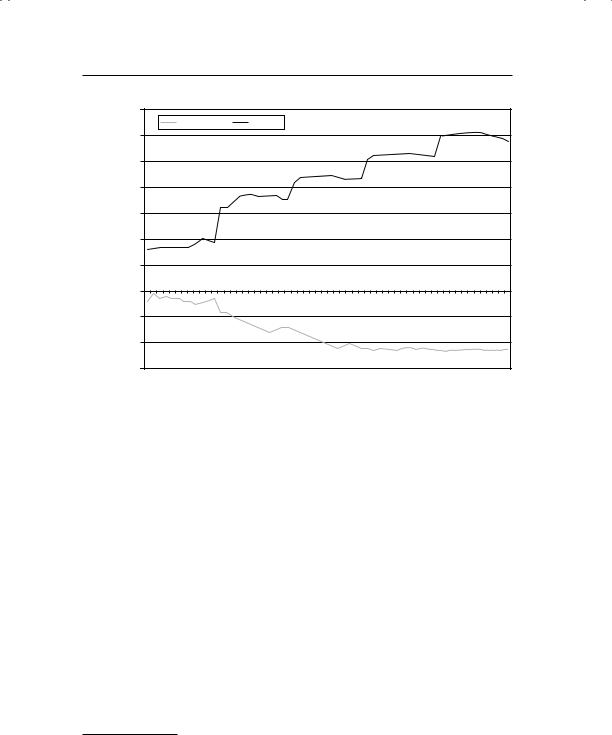
F I G U R E 8 . 4 Returns on Dividend Yield Classes, 1952 to 2010
Source: Raw data from Ken French’s Data Library (Dartmouth College).
that they generate excess returns from it, but they compare the returns to what you would have made on the Dow 30 and the S&P 500 and do not adequately adjust for risk. A portfolio with only 10 stocks in it is likely to have a substantial amount of firm-specific risk. McQueen, Shields, and Thorley examined this strategy and concluded that while the raw returns from buying the top dividend-paying stocks are higher than the rest of the index, adjusting for risk and taxes eliminates all of the excess return.16 A later study by Hirschey also indicates that there are no excess returns from this strategy after you adjust for risk.17
There are three final considerations in a high-dividend strategy. The first is that you will have a much greater tax cost on this strategy, if dividends are taxed at a higher rate than capital gains. That was the case prior to 2003 and may very well be true again starting in 2013. The second is that some
16G. McQueen, K. Shields, and S. R. Thorley, “Does the Dow-10 Investment Strategy Beat the Dow Statistically and Economically?” Financial Analysts Journal (July/August 1997): 66–72.
17M. Hirschey, “The ‘Dogs of the Dow’ Myth,” Financial Review 35 (2000): 1–15.

Graham’s Disciples: Value Investing |
281 |
stocks with high dividend yields may be paying much more in dividends than they can afford and the market is building in the expectation of a dividend cut, into the stock price. The third is that any stock that pays a substantial portion of its earnings as dividends is reinvesting less and can therefore expect to grow at a much lower rate.
D e t e r m i n a n t s o f S u c c e s s
If all we have to do to earn excess returns is invest in stocks that trade at low multiples of earnings, book value, or revenues, shouldn’t more investors employ these screens to pick their portfolios? And assuming that they do, should they not beat the market by a healthy amount?
To answer the first question, a large number of portfolio managers and individual investors employ either the screens we have referred to in this section or variants of these screens to pick stocks. Unfortunately, their performance does not seem to match up to the returns that we see earned on the hypothetical portfolios. Why might that be? We can think of several reasons.
Time horizon. All of the studies quoted earlier look at returns over time horizons of five years or greater. In fact, low price-to-book value stocks have underperformed high price-to-book value stocks over shorter time periods. The same can be said about P/E ratios and price-to-sales ratios.
Dueling screens. If one screen earns you excess returns, three should do even better seems to be the attitude of some investors who proceed to multiply the screens they use. They are assisted in this process by the easy access to both data and screening technology. There are websites (many of which are free) that allow you to screen stocks (at least in the United States) using multiple criteria.18 The problem, though, is that the use of one screen may undercut the effectiveness of others, leading to worse rather than better portfolios.
Absence of diversification. In their enthusiasm for screens, investors sometimes forget the first principles of diversification. For instance, it is not uncommon to see stocks from one sector disproportionately represented in portfolios created using screens. A screen from low-P/E stocks may deliver a portfolio of banks and utilities, whereas a screen of low price-to-book ratios and high returns on equity may deliver stocks
18Stockscreener.com, run by Hoover, is one example. You can screen all listed stocks in the United States using multiple criteria, including all of the criteria discussed in this chapter.

282 |
INVESTMENT PHILOSOPHIES |
from a sector with high infrastructure investments that has had bad sector-specific news come out about it.
Taxes and transaction costs. As in any investment strategy, taxes and transaction costs can take a bite out of returns, although the effect should become smaller as your time horizon lengthens. Some screens, though, can increase the effect of taxes and transaction costs. For instance, screening for stocks with high dividends and low P/E ratios will yield a portfolio that may have much higher tax liabilities (because of the dividends).
Success and imitation. In some ways, the worst thing that can occur to a screen (at least from the viewpoint of investors using the screen) is that its success is publicized and that a large number of investors begin using that same screen at the same time. In the process of creating portfolios of the stocks they perceive to be undervalued, they may very well eliminate the excess returns that drew them to the screen in the first place.
To be a successful screener, you would need to be able to avoid or manage these problems. In particular, you need to have a long time horizon, pick your combination of screens well, and ensure that you are reasonably diversified. If a screen succeeds, you will probably need to revisit it at regular intervals to ensure that market learning has not reduced the efficacy of the screen.
T o o l s f o r S u c c e s s
Passive value investors know that there are no sure winners in investing. Buying low P/E or low price-to-book value ratios may have generated high returns in the past but there are pitfalls in every strategy. Since value investors are bound by a common philosophy, which is that you should minimize your downside risk without giving up too much of your upside potential, they have devised tools to put this philosophy into practice in the past few decades.
A c c o u n t i n g C h e c k s The two most widely used multiples used to find cheap stocks, P/E and price-to-book ratios, both have accounting numbers in the denominator—accounting earnings in the case of P/E, and accounting book value in the case of price-to-book. To the extent that these accounting numbers are unsustainable, manipulated, or misleading, the investment choices that follow will reflect these biases. Thus, a company that reports inflated earnings, either because it had an unusually good year (a commodity company after a spike in the price of the commodity) or because of accounting choices (which can range from discretion within the accounting rules to

Graham’s Disciples: Value Investing |
283 |
fraud), will look cheap on a price-earnings ratio basis. Similarly, a firm that takes a large restructuring charge and writes down its book value of assets (and equity) will look expensive on a price-to-book basis.
To combat the problem, value investors have developed ways of correcting both earnings and book value. With accounting earnings, there are three widely used alternatives to the actual earnings. The first is normalized earnings, where value investors look at the average earnings earned over a fiveor 10-year period rather than earnings in the most recent year. With commodity and cyclical companies, this will allow for smoothing out of cycles and result in earnings that are much lower than actual earnings (if earnings are at a peak) or higher than actual earnings (if earnings have bottomed out). The second is adjusted earnings, where investors who are willing to delve through the details of company filings and annual reports often devise their own measures of earnings that correct for what they see as shortcomings in conventional accounting earnings. The adjustments usually include eliminating one-time items (income and expenses) and estimating expenses for upcoming liabilities (underfunded pension or health care costs). Finally, we noted Buffett’s use of a modified version of owner’s earnings, where depreciation, amortization, and other noncash charges are added back and capital expenditures needed to maintain existing assets are subtracted out to get to “owners’ earnings.” In effect, this replaces earnings with a cash flow after maintenance investments have been made.
With book value, value investors have to deal with two problems. The first is that the book value of a company’s assets and equity will generally be inflated after it acquires another company, because you are required to show the price you paid and the resulting goodwill as an asset. Netting goodwill out of assets will reduce book value and make acquisitive companies look less attractive on a price-to-book basis. Consequently, value investors often use tangible book value, rather than total book value, where
Tangible book value = Book value − Goodwill − Other intangible assets
The second is that book value does not equate to liquidation value; in other words, some assets are easier to liquidate (and convert to cash at or close to their book value) than other assets. To compensate for the difficulty of converting book value to cash for some assets, value investors also look at narrower measures of book value with greater weight given to liquid assets. In one of its most conservative versions, some value investors look at only current assets (on the assumption that accounts receivable and inventory can be more easily sold at close to book value) and compute a net net value (Book value of current assets – Book value of current liabilities – Book value of long-term debt). Buying a company for less than its net net value is thus

284 |
INVESTMENT PHILOSOPHIES |
considered an uncommon bargain, since you can liquidate its current assets, pay off its outstanding liabilities, and pocket the difference.
T h e M o a t When you buy a stock at a low price-earnings ratio or because it has a high dividend yield, you are implicitly assuming that it can continue generating these earnings (and paying dividends) in the long term. For this to occur, the firm has to be able to hold on to (and hopefully even strengthen) its market share and margins in the face of competition. The “moat” is a measure of a company’s competitive advantages; the stronger and more sustainable a company’s competitive advantages, the more difficult it becomes for others to breach the moat and the safer the earnings stream becomes.
But how do you measure this moat? Some value investors look at the company’s history, arguing with some legitimacy that a history of stable earnings and steady growth is evidence of a deep moat. Others use qualitative factors, such as the presence of an experienced and competent management team, the possession of a powerful brand name, or the ownership of a license or patent. With either approach, the objective is to look at the underpinnings of reported earnings to see if they can be sustained in the future.
M a r g i n o f S a f e t y In Chapter 2, we included an extensive section on margin of safety. Summarizing, the margin of safety (MOS) is the buffer that value investors build into their investment decision to protect themselves against risk. Thus, a MOS of 20 percent would imply that an investor would buy a stock only if its price is more than 20 percent below the estimated value (estimated using a multiple or a discounted cash flow model).
Value investors use the margin of safety as their protection from being wrong on two levels. The first is in their assessment of the intrinsic value of a company, where the errors can come from erroneous assumptions about the future of the company or unforeseen macroeconomic risks. The second is in the market price adjustment; after all, there is no guarantee that the stock price will move toward the intrinsic value, even if the intrinsic value is right. Extending the logic, the margin of safety should be larger for riskier companies where there is more uncertainty about the future. It should also widen during periods of market crisis, when macroeconomic risks become larger, and in inefficient or illiquid markets, where the price adjustment may take more time.
T H E C O N T R A R I A N V A L U E I N V E S T O R
The second strand of value investing is contrarian value investing. In this manifestation of value investing, you begin with the belief that stocks that

Graham’s Disciples: Value Investing |
285 |
are beaten down because of the perception that they are poor investments (because of their own poor investments, default risk, or bad management) tend to get punished too much by markets, just as stocks that are viewed as good investments get pushed up too much. Within contrarian investing, we would include several strategies ranging from relatively unsophisticated ones like buying the biggest losers in the market in the prior period to vulture and distressed security investing, where you use sophisticated quantitative techniques to highlight securities (both stocks and bonds) issued by troubled firms that may be undervalued.
B a s i s f o r C o n t r a r i a n I n v e s t i n g
Do markets overreact to new information and systematically overprice stocks when the news is good and underprice stocks when the news is bad? There is some evidence for this proposition, especially in the long term, and, as we noted in Chapter 7, studies do find that stocks that have done exceptionally well or badly in a period tend to reverse course in the following period, but only if the period is defined in terms of years rather than weeks or months.
S t r a t e g i e s a n d E v i d e n c e
Contrarian investing takes many forms, but we will consider just three strategies in this section. We will begin with the simple strategy of buying stocks that have gone down the most over the previous period; move on to a slightly more sophisticated process of playing the expectations game, buying stocks where expectations have been set too low and selling stocks where expectations are too high; and end the section by looking at a strategy of investing in securities issued by firms in significant operating and financial trouble.
B u y i n g t h e L o s e r s In Chapter 7, we presented evidence that stocks reverse themselves over long periods in the form of negative serial correlation; that is, stocks that have gone up the most over the past five years are more likely to go down over the next five years. Conversely, stocks that have gone down the most over the past five years are more likely to go up. In this section, we consider a strategy of buying the latter and selling or avoiding the former.
The Evidence How would a strategy of buying the stocks that have gone down the most over the past few years perform? To isolate the effect of price reversals on the extreme portfolios, DeBondt and Thaler constructed a winners portfolio of 35 stocks that had gone up the most over the prior year, and a losers portfolio of 35 stocks that had gone down the most over
286 |
|
|
|
|
|
|
|
|
|
|
|
INVESTMENT PHILOSOPHIES |
|||||||
|
35.00% |
|
|
|
|
|
|
|
|
|
|
|
|
|
|
|
|
|
|
|
30.00% |
|
Winners |
Losers |
|
|
|
|
|
|
|
|
|
|
|
|
|||
|
|
|
|
|
|
|
|
|
|
|
|
|
|
|
|
|
|
|
|
|
25.00% |
|
|
|
|
|
|
|
|
|
|
|
|
|
|
|
|
|
|
Return |
20.00% |
|
|
|
|
|
|
|
|
|
|
|
|
|
|
|
|
|
|
|
|
|
|
|
|
|
|
|
|
|
|
|
|
|
|
|
|
|
|
Abnormal |
15.00% |
|
|
|
|
|
|
|
|
|
|
|
|
|
|
|
|
|
|
10.00% |
|
|
|
|
|
|
|
|
|
|
|
|
|
|
|
|
|
|
|
|
|
|
|
|
|
|
|
|
|
|
|
|
|
|
|
|
|
|
|
Cumulative |
5.00% |
|
|
|
|
|
|
|
|
|
|
|
|
|
|
|
|
|
|
0.00% |
|
|
|
|
|
|
|
|
|
|
|
|
|
|
|
|
|
|
|
–5.00% |
|
|
|
|
|
|
|
|
|
|
|
|
|
|
|
|
|
|
|
|
|
|
|
|
|
|
|
|
|
|
|
|
|
|
|
|
|
|
|
|
–10.00% |
|
|
|
|
|
|
|
|
|
|
|
|
|
|
|
|
|
|
|
–15.00% |
|
|
|
|
|
|
|
28 |
|
|
37 |
40 |
|
|
|
|
|
58 |
|
1 |
4 |
7 |
10 |
13 16 |
19 |
22 |
25 |
31 |
34 |
43 |
46 |
49 |
52 |
55 |
||||
Months after Portfolio Formation
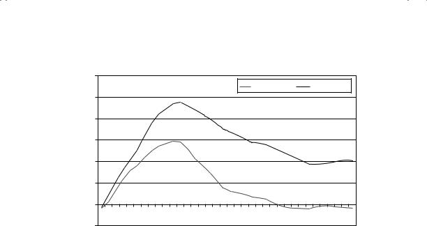
F I G U R E 8 . 5 Cumulative Abnormal Returns—Winners versus Losers
Source: W. F. M. DeBondt and R. Thaler, “Further Evidence on Investor Overreaction and Stock Market Seasonality,” Journal of Finance 42 (1987): 557–581.
the prior year, each year from 1933 to 1978.19 They examined returns on these portfolios for the 60 months following the creation of the portfolio. Figure 8.5 graphs the returns on both the loser and winner portfolios.
This analysis suggests that an investor who bought the 35 biggest losers over the previous year and held for five years would have generated a cumulative abnormal return of approximately 30 percent over the market and about 40 percent over an investor who bought the winners portfolio.
This evidence is consistent with market overreaction and suggests that a simple strategy of buying stocks that have gone down the most over the past year or years may yield excess returns over the long term. Since the strategy relies entirely on past prices, you could argue that this strategy shares more with charting (consider it a long-term contrarian indicator) than it does with value investing.
19W. F. M. DeBondt and R. Thaler, “Further Evidence on Investor Overreaction and Stock Market Seasonality,” Journal of Finance 42 (1987): 557–581.

Graham’s Disciples: Value Investing |
287 |
Caveats There are many academics as well as practitioners who suggest that these findings are interesting but that they overstate potential returns on loser portfolios for several reasons:
There is evidence that loser portfolios are more likely to contain lowpriced stocks (selling for less than $5), which generate higher transaction costs and are also more likely to offer heavily skewed returns; that is, the excess returns come from a few stocks making phenomenal returns rather than from consistent performance.
Studies also seem to find that loser portfolios created every December earn significantly higher returns than portfolios created every June. This suggests an interaction between this strategy and tax-loss selling by investors. Since stocks that have gone down the most are likely to be sold toward the end of each tax year (which ends in December for most individuals), their prices may be pushed down by the tax-loss selling.
There seems to be a size effect when it comes to the differential returns. When you do not control for firm size, the loser stocks outperform the winner stocks; but when you match losers and winners of comparable market value, the only month in which the loser stocks outperform the winner stocks is January.20
The final point to be made relates to time horizon. As we noted in the preceding chapter, while there may be evidence of price reversals in long periods (three to five years), there is evidence of price momentum (losing stocks are more likely to keep losing and winning stocks to keep winning) if you consider shorter periods (six months to a year). An earlier study that we referenced, by Jegadeesh and Titman, tracked the difference between winner and loser portfolios by the number of months that you held the portfolios.21 Their findings are summarized in Figure 8.6.
There are two interesting findings in this graph. The first is that the winner portfolio actually outperforms the loser portfolio in the first 12 months. The second is that while loser stocks start gaining ground on winning stocks after 12 months, it took them 26 months in the 1941–1964 time
20P. Zarowin, “Size, Seasonality and Stock Market Overreaction,” Journal of Financial and Quantitative Analysis 25 (1990): 113–125.
21N. Jegadeesh and S. Titman, “Returns to Buying Winners and Selling Losers: Implications for Stock Market Efficiency,” Journal of Finance 48, no. 1 (1993): 65–91.
288 |
INVESTMENT PHILOSOPHIES |
Cumulative Abnormal Return (Winner – Loser)
12.00%
1941–1964 |
1965–1989 |
10.00%
8.00%
6.00%
4.00%
2.00%
0.00%
1 |
2 |
3 |
4 |
5 |
6 |
7 |
8 |
9 10 11 12 13 14 15 16 17 18 19 20 21 22 23 24 25 26 27 28 29 30 31 32 33 34 3536 |
–2.00%
Months after Portfolio Formation
F I G U R E 8 . 6 Differential Returns—Winner versus Loser Portfolios
Source: N. Jegadeesh and S. Titman, “Returns to Buying Winners and Selling Losers: Implications for Stock Market Efficiency,” Journal of Finance 48, no. 1 (1993): 65–91.
period to get ahead of them, and the loser portfolio does not start outperforming the winner portfolio even with a 36-month time horizon in the 1965–1989 time period. The payoff to buying losing companies may depend heavily on whether you have the capacity to hold these stocks for long time periods.
P l a y i n g t h e E x p e c t a t i o n s G a m e A more sophisticated version of contrarian investing is to play the expectations game. If you are right about markets overreacting to recent events, expectations will be set too high for stocks that have been performing well and too low for stocks that have been doing badly. If you can isolate these companies, you can buy the latter and sell the former. In this section, we consider a couple of ways in which you can invest on expectations.
Bad Companies Can Be Good Investments Any investment strategy that is based on buying well-run, good companies and expecting the growth in earnings in these companies to carry prices higher is dangerous, since it ignores the possibility that the current price of the company already reflects the quality of the management and the firm. If the current price is right (and the market is paying a premium for quality), the biggest danger is that the

Graham’s Disciples: Value Investing |
289 |
|
T A B L E 8 . 2 Excellent versus Unexcellent Companies—Financial Comparison |
||
|
|
|
|
Excellent Companies |
Unexcellent Companies |
|
|
|
Growth in assets |
10.74% |
4.77% |
Growth in equity |
9.37% |
3.91% |
Return on capital |
10.65% |
1.68% |
Return on equity |
12.92% |
−15.96% |
Net margin |
6.40% |
1.35% |
firm loses its luster over time and the premium paid will dissipate. If the market is exaggerating the value of the firm, this strategy can lead to poor returns even if the firm delivers its expected growth. It is only when markets underestimate the value of firm quality that this strategy stands a chance of making excess returns.
There is some evidence that well-managed companies do not always make good investments. Tom Peters, in his widely read book on excellent companies a few years ago, outlined some of the qualities that he felt separated excellent companies from the rest of the market.22 Without contesting his standards, a study went through the perverse exercise of finding companies that failed on each of the criteria for excellence—a group of unexcellent companies—and contrasting them with a group of excellent companies. Table 8.2 provides summary statistics for both groups.23
The excellent companies clearly are in much better financial shape and are more profitable than the unexcellent companies, but are they better investments? Figure 8.7 contrasts the returns that would have been made on these companies versus the excellent ones.
The excellent companies may be in better shape financially, but the unexcellent companies would have been much better investments, at least over the time period considered (1981–1985). An investment of $100 in unexcellent companies in 1981 would have grown to $298 by 1986, whereas $100 invested in excellent companies would have grown to only $182. While this study did not control for risk, it does present some evidence that good companies are not necessarily good investments, whereas bad companies can sometimes be excellent investments.
The second study used a more conventional measure of company quality. Standard & Poor’s, the ratings agency, assigns quality ratings to stocks
22T. Peters, In Search of Excellence: Lessons form America’s Best Run Companies
(New York: Warner Books, 1988).
23M. Clayman, “Excellence Revisited,” Financial Analysts Journal (May/June 1994): 61–66.