aswath_damodaran-investment_philosophies_2012

F I G U R E 7 . 1 Information and Price Changes in a Rational Market

of abuse from technical analysts, some justified and some not, we will begin by looking at what the random walk is and its implications.

T h e B a s i s f o r R a n d o m W a l k s

To understand the argument for prices following a random walk, we have to begin with the presumption that investors at any point in time estimate the value of an asset based on expectations of the future, and that these expectations are both unbiased and rational, given the information that investors have at that point in time. Under these conditions, the price of the asset changes only as new information comes out about it. If the market price at any point in time is an unbiased estimate of value, the next piece of information that comes out about the asset should be just as likely to contain good news as bad.1 It therefore follows that the next price change is just as likely to be positive as it likely to be negative. The implication of course is that each price change will be independent of the previous one, so knowing an asset’s price history will not help form better predictions of future price changes. Figure 7.1 summarizes the assumptions.

The random walk is not magic, but there are two prerequisites for it to hold. The first is that investors are rational and form unbiased expectations of the future, based on all of the information that is available to them at the

1If the probability of good news is greater than the probability of bad news, the price should increase before the news comes out. Technically, it is the expected value of the next information release that is zero.

time. If expectations are set too low or set too high consistently—in other words, investors are too optimistic or too pessimistic—information will no longer have an equal chance of being good or bad news, and prices will not follow a random walk. The second is that price changes are caused by new information. If investors can cause prices to change by just trading, even in the absence of information, you can have price changes in the same direction rather than a random walk.

T h e B a s i s f o r P r i c e P a t t e r n s

Chartists are not alone in believing that there is information in past prices that can be useful in forecasting future price changes. There are some fundamental investors who use technical and charting indicators, albeit as secondary factors, in picking stocks. They disagree with the basic assumptions made by random walkers and argue that:

Investors are not always rational in the way they set expectations. These irrationalities may lead to expectations being set too low for some assets at some times and too high for other assets at other times. Thus, the next piece of information is more likely to contain good news for the first asset and bad news for the second.

Price changes themselves may provide information to markets. Thus, the fact that a stock has gone up strongly the past four days may be viewed as good news by investors, making it more likely that the price will go up today rather than down.

The debate about whether price changes are random has continued for the past 50 years, ever since researchers were able to access price data on stocks. The initial tests were almost all conducted by those who believed that prices follow a random walk, and, not surprisingly, they found no price patterns. In the past two decades, there has been an explosion in both the amount of data available and in the points of view of researchers. One of the biggest surprises (at least to those who believed the prevailing dogma of efficient and rational markets) has been the uncovering of numerous price patterns, though it is not clear whether these are evidence of irrational markets and whether they offer the potential for profits.

E M P I R I C A L E V I D E N C E

As the studies of the time series properties of prices have proliferated, the evidence can be classified based on the periods over which researchers examine

expected in a series of this length, assuming that price changes are random.8 If the actual number of runs is greater than the expected number, there is evidence of negative correlation in price changes. If it is lower, there is evidence of positive correlation. A study of price changes in the Dow 30 stocks, assuming daily, four-day, nine-day, and 16-day return intervals, provided the following results.

The actual number of runs in four-day returns (175.7) is almost exactly what you would expect in a random process. There is slight evidence of positive correlation in daily returns but no evidence of deviations from randomness for longer return intervals.

Again, while the evidence is dated, it serves to illustrate the point that long strings of positive and negative changes are, by themselves, insufficient evidence that markets are not random, since such behavior is consistent with price changes following a random walk. It is the recurrence of these strings that can be viewed as evidence against randomness in price behavior.

H I G H - F R E Q U E N C Y T R A D I N G

High-frequency trading generally references automated trading, usually in high volume, often by institutional investors. While that may not sound unique or even new, high-frequency trading is entirely driven by computer algorithms, rather than by human insight or decisions.

Thus, if there are patterns in stock prices and information in trading volume, even over very short time periods, computer algorithms can be written to instantaneously take advantage of these patterns to make money. While the profits generated per share may be tiny, they can amount to sizable values over very large trades.

(continued)

8There are statistical tables that summarize the expected number of runs, assuming randomness, in a series of any length.

High-frequency trading has created its own share of headlines, most of which have been negative. It has been blamed for so-called flash crashes, where a mistake in the computer algorithm or faulty data can result in price instability. A drop in U.S. stocks of almost 5 percent during a 30-minute period on May 6, 2010, for instance, was at least partially attributed to high-frequency trading in index futures. It has also become as a symbol of how uneven the playing field is for individual investors, who do not have the resources for high-frequency trading and have to compete with institutional investors who do.

We believe that the criticism is overblown. First, high-frequency trading has exacerbated some of the volatility in markets, but the rise in stock market volatility in the post-2008 time period has more to do with increases in macroeconomic uncertainty than with trading mechanisms. Second, individual investors should never be trying to exploit minute-to-minute movements in stock prices in the first place, with or without high-frequency trading. As for the institutional investors who use high-frequency trading, it is possible that the first entrants in this game claimed some surplus from short-term price movements, but as it has become more common, the payoff has become more modest.

T h e S h o r t T e r m : P r i c e R e v e r s a l As you move from hours and days to weeks or months, there seems to be some evidence that prices reverse. In other words, stocks that have done well over the last month are more likely to do badly in the next one, and stocks that have done badly over the last month are more likely to bounce back.9 The reasons given are usually rooted in market overreaction; the stocks that have gone up (or down) the most over the most recent month are ones where markets have overreacted to good (or bad) news that came out about the stock over the month. The price reversal then reflects markets correcting themselves.

A study looked at the differential returns that would have been generated by a strategy of selling short the top decile of stocks based on how well they did in the past month, and buying the stocks in the bottom decile, with a

9N. Jegadeesh, “Evidence of Predictable Behavior of Security Returns,” Journal of Finance 45 (1990): 881–898; B. N. Lehmann, “Fads, Martingales, and Market Efficiency,” Quarterly Journal of Economics 105 (1990): 1–28.

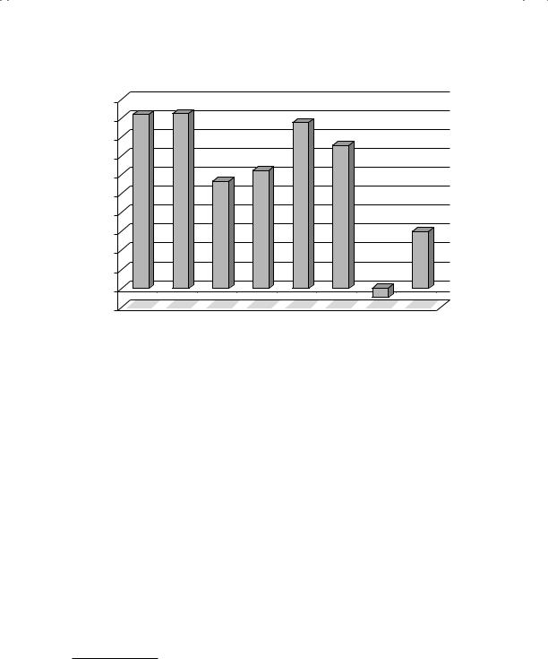
F I G U R E 7 . 2 Annual Returns to Short-Term Reversal Strategy, 1929 to 2009 Source: D. Blitz, J. Huij, S. Lansdorp and M. Verbeek, “Short-Term Residual Return” (SSRN Working Paper 1911449, 2010).

holding period of a month.10 The annualized returns from this strategy are presented in Figure 7.2. The strategy would have generated substantial profits, before adjusting for transaction costs and risk, in all but one decade (1989–1999) out of the last eight decades.

Studies that have looked at short-term price reversal do present three caveats that should play a role in whether you should invest based on the phenomenon. The first is that this strategy can skew toward buying small market cap companies with low price-to-book ratios, at least in some periods. To the extent that these companies are riskier, the excess returns on this strategy have to be scaled down. The second is that this is a high trading/turnover strategy and the transaction costs can eat into the excess returns significantly, especially if the stocks being traded are small market cap companies. The third is that to the extent that this is a strategy built around market overreaction to news, it may be more effective to build it around actual news announcements. For instance, we will look at a strategy of trading after earnings announcements in Chapter 10 that represents a much more direct way of exploiting market overreaction.

10D. Blitz, J. Huij, S. Lansdorp, and M. Verbeek, “Short-Term Residual Return” (SSRN Working Paper 1911449, 2010).

T h e M i d T e r m : P r i c e M o m e n t u m

When time is defined as many months or a year rather than a single month, there seems to be a tendency toward positive serial correlation. Jegadeesh and Titman present evidence of what they call “price momentum” in stock prices over time periods of several months—stocks that have gone up in the past six months tend to continue to go up, whereas stocks that have gone down in the past six months tend to continue to go down.11 Between 1945 and 2008, if you classified stocks into deciles based on price performance over the previous year, the annual return you would have generated by buying the stocks in the top decile and holding for the next year was 16.5 percent higher than the return you would have earned on the stocks in the bottom decile. To add to the allure of the strategy, the high-momentum stocks also had less risk (measured as price volatility) than the low-momentum stocks.12

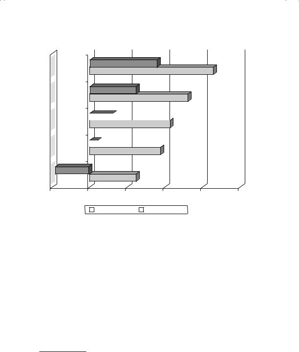
Figure 7.3 shows the allure to a momentum strategy by looking at the annual returns, from 1927 to 2010, to investing in stocks classified into momentum classes based on the most recent year’s performance.

The momentum effect is just as strong in the European markets, though it seems to be weaker in emerging markets.13 In the United Kingdom, Dimson, Marsh, and Staunton looked at the 100 largest stocks on the British market and compared the value of a portfolio composed of the 20 best performers over the previous 12 months with the 20 worst performers over the same period; £1 invested in the best performers in 1900 would have grown to £2.3 million at the end of 2009, whereas £1 invested in the worst performers would have grown to only £49.

What may cause this momentum? One potential explanation is that mutual funds are more likely to buy past winners and dump past losers, and they tend to do this at the same time, thus generating price continuity.14 In

11N. Jegadeesh and S. Titman, “Returns to Buying Winners and Selling Losers: Implications for Stock Market Efficiency,” Journal of Finance 48, no. 1 (1993): 65–91; N. Jegadeesh and S. Titman, “Profitability of Momentum Strategies: An Evaluation of Alternative Explanations,” Journal of Finance 56, no. 2 (2001): 699–

12K. Daniel, “Momentum Crashes” (SSRN Working Paper 1914673, 2011).

13G. K. Rouwenhorst, “International Momentum Strategies,” Journal of Finance 53 (1998): 267–284; G. Bekaert, C. B. Erb, C. R. Harvey, and T. E. Viskanta, “What Matters for Emerging Market Equity Investments,” Emerging Markets Quarterly (Summer 1997): 17–46.

14M. Grinblatt, S. Titman, and R. Wermers, “Momentum Investment Strategies,

Portfolio Performance, and Herding: A Study of Mutual Fund Behavior,” American Economic Review 85 (1995): 1088–1105.

Biggest

winners

Momentum

4

Momentum

3

Momentum

2

Biggest

losers

F I G U R E 7 . 3 Annual Returns to Momentum from 1927 to 2010—U.S. Stocks Momentum Classes Based on Prior Year’s Performance

Source: Raw data from Ken French’s Data Library (Dartmouth College).

recent years, as more research has been done on the momentum effect, four interesting patterns are emerging:

1.Price momentum that is accompanied by higher trading volume is both stronger and more sustained than price momentum with low trading volume.15

2.There are differences in opinion on the relationship between momentum and firm size. While some of the earlier studies suggest that momentum is stronger at small market cap companies, a more recent study that looks at U.S. stocks from 1926 to 2009 finds the relationship to be a weak

15K. Chan, A. Hameed, and W. Tong, “Profitability of Momentum Strategies in the International Equity Markets,” Journal of Financial and Quantitative Analysis 35 (2000): 153–172.