

aswath_damodaran-investment_philosophies_2012
.pdf230 |
INVESTMENT PHILOSOPHIES |
Another may be that it is far easier to create investment strategies to take advantage of an underpriced asset than it is to take advantage of an overpriced one. With the former, you can always buy the asset and hold until the market rebounds. With the latter, your choices are both more limited and more likely to be time limited. You can borrow the asset and sell it (short the asset), but not for as long as you want—most short selling is for a few months. If there are options traded on the asset, you may be able to buy puts on the asset, though until recently, only of a few months’ duration. In fact, there is a regulatory bias in most markets against such investors, who are often likely to be categorized as speculators. As a consequence of these restrictions on betting against overpriced assets, bubbles on the upside are more likely to persist and become bigger over time, whereas bargain hunters operate as a floor for downside bubbles.
A C l o s i n g A s s e s s m e n t Based on our reading of history, it seems reasonable to conclude that there are bubbles in asset prices, though only some of them can be attributed to market irrationality. Whether investors can take advantage of bubbles to make money seems to be a more difficult question to answer. One reason for the failure to exploit bubbles seems to stem from the desire to partake in the short term profits; even investors who believe that assets are overpriced want to make money off the bubble. Another reason is that it is difficult and dangerous to go against the crowd. Overvalued assets may get even more overvalued and these overvaluations can stretch over years, thus imperiling the financial well-being of any investor who has bet against the bubble. Finally, there is also an institutional interest on the part of investment banks, the media, and portfolio managers, all of whom feed of the bubble, to perpetuate the bubble.
S e a s o n a l a n d T e m p o r a l P a t t e r n s i n P r i c e s
One of the most puzzling phenomena in asset prices is the existence of seasonal and temporal patterns in stock prices that seem to cut across all types of asset markets. As we will see in this section, stock prices seem to go down more on Mondays than on any other day of the week and do better in January than in any other month of the year. What is so surprising about this phenomenon, you might ask? It is very difficult to justify the existence of patterns such as these in a rational market; after all, if investors know that stocks do better in January than in any other month, they should start buying the stock in December and shift the positive returns over the course of the year. Similarly, if investors know that stocks are likely to be marked down on Monday, they should begin marking them down on Friday and hence shift the negative returns over the course of the week.
Smoke and Mirrors? Price Patterns, Volume Charts, and Technical Analysis |
231 |
4.50% |
|
|
|
|
|
|
|
|
Entire Market |
|
|
|
|
|
|
|
|
|
|
||
4.00% |
|
|
|
|
|
|
|
|
|
|
3.50% |
|
|
|
|
|
|
|
|
|
|
3.00% |
|
|
|
|
|
|
|
|
|
|
2.50% |
|
|
|
|
|
|
|
|
|
|
2.00% |
|
|
|
|
|
|
|
|
|
|
1.50% |
|
|
|
|
|
|
|
|
|
|
1.00% |
|
|
|
|
|
|
|
|
|
|
0.50% |
|
|
|
|
|
|
|
|
|
|
0.00% |
|
|
|
|
|
|
|
|
|
|
|
January |
February |
March |
April |
May |
June |
y |
August |
October |
November December |
–0.50% |
Jul |
|||||||||
|
|
|
|
|
||||||
|
|
|
|
|
|
|
September |
|
||
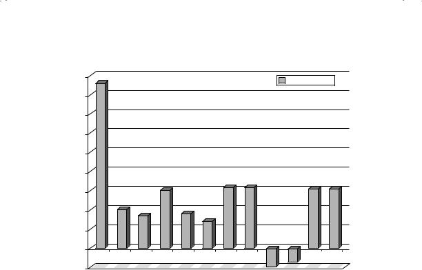
F I G U R E 7 . 9 Returns by Month of the Year: U.S. Stocks from 1927 to 2011 Source: Raw data from Ken French’s Data Library (Dartmouth College).
T h e J a n u a r y E f f e c t Studies of returns in the United States and other major financial markets consistently reveal strong differences in return behavior across the months of the year. Figure 7.9 reports average returns by month of the year from 1927 to 2011.
Returns in January are significantly higher than returns in any other month of the year. This phenomenon is called the year-end or January effect, and it can be traced specifically to the first two weeks in January.
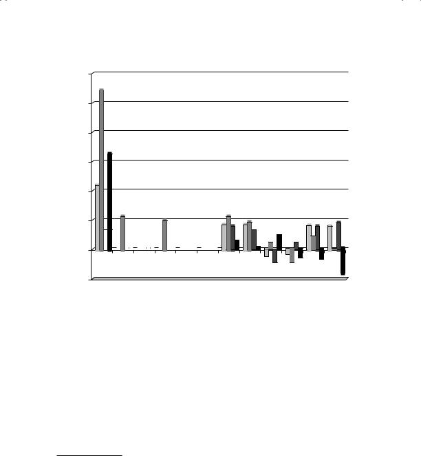
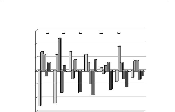
The January effect is much more pronounced for small firms than for larger firms, and Figure 7.10 graphs returns in January for the smallest firms (bottom 10 percent), the largest firms (top 10 percent) and the small cap premium (the difference between the smallest company returns and the entire market) from 1927 to 2011. We will return to examine this phenomenon in Chapter 9, where we take a closer look at investing in small-cap stocks as a strategy.
Note that the bulk of the small cap premium is earned in January and that small-cap stocks underperform the market for last quarter of each calendar year.
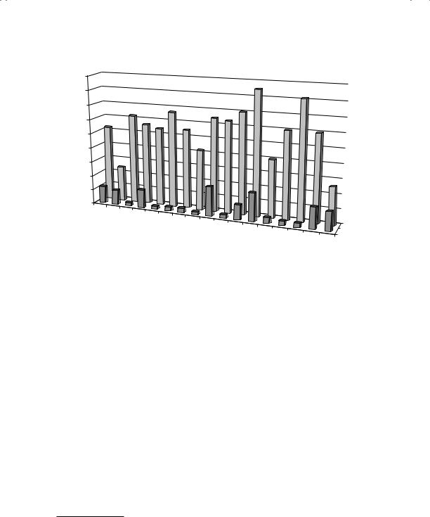
The universality of the January effect is illustrated in Figure 7.11, which reports on returns in January versus the other months of the year in several
232 |
|
|
|
|
|
INVESTMENT PHILOSOPHIES |
|||
12.00% |
|
|
|
|
|
|
|
|
|
|
|
|
|
|
Entire Market |
|
|
Largest Market Cap |
|
10.00% |
|
|
|
|
Smallest Market Cap |
|
Premium over Market |
|
|
|
|
|
|
|
|
||||
|
|
|
|
|
|
|
|
|
|
|
|
|
|
|
|
|
|
|
|
8.00%
6.00%
4.00%
2.00%
0.00% |
|
|
|
|
|
|
|
|
|
|
|
|
|
|
|
|
|
|
|
|
|
|
|
|
|
|
|
|
|
|
|
|
|
|
|
|
|
|
|
|
|
|
|
|
|
|
|
|
|
|
|
|
|
|
|
|
|
|
|
|
|
|
|
|
|
|
|
|
|
|
|
|
|
|
|
|
|
|
|
|
|
|
|
|
|
|
|
|
|
|
|
|
|
|
|
|
|
|
|
|
|
|
|
|
|
|
|
|
|
|
|
|
|
|
|
|
|
|
|
|
|
|
|
|
|
|
|
|
|
|
|
|
|
|
|
|
|
|
|
|
|
|
|
|
|
|
|
|
|
|
|
|
|
|
|
|
|
|
|
|
|
|
|
|
|
|
|
|
|
|
|
|
|
January |
|
March April |
|
|
|
|
|
|
|
|
|
|
|
|
||||||||||||||
–2.00% |
February |
|
|
|
May |
|
|
June |
|
|
||||||||||||||||||
|
|
|
|
|
|
|
|
|
|
|
|
|
|
|
|
|
|
|
|
|
|
|||||||
July |
August |
October |
|
September |
|
|
NovemberDecember |
F I G U R E 7 . 1 0 Small Cap Premium by Month of Year: U.S. Stocks from 1927 to 2011
Source: Raw data from Ken French’s Data Library (Dartmouth College).
major financial markets, and finds strong evidence of a January effect in every market.22
In fact, researchers have unearthed evidence of a January effect in bond and commodity markets as well as stocks.
A number of explanations have been advanced for the January effect, but few hold up to serious scrutiny. One is that there is tax-loss selling by investors at the end of the year on stocks that have gone down to capture the capital gain, driving prices further down, presumably below true value, in December, and a buying back of the same stocks in January, resulting in the high returns.23 The fact that the January effect is accentuated for
22R. Haugen and J. Lakonishok, The Incredible January Effect (Homewood, IL: Dow-Jones Irwin, 1988).
23It is to prevent this type of trading that the Internal Revenue Service has a “wash sale rule” that prevents you from selling and buying back the same stock within
45days. To get around this rule, there has to be some substitution among the stocks. Thus investor 1 sells stock A and investor 2 sells stock B, but when it comes time to
buy back the stock, investor 1 buys stock B and investor 2 buys stock A.
Smoke and Mirrors? Price Patterns, Volume Charts, and Technical Analysis |
233 |
Average Monthly Return
4.50%
4.00%
3.50%
3.00%
2.50%
2.00%
1.50%
1.00%
0.50%
0.00%
Australia |
|
|
|
|
|
|
|
|
|
|
Austria |
|
|
|
|
|
|
|
|
|
|
Belgium |
France |
Italy |
|
nds |
|
|
|
|
|
|
Canada |
Japan |
|
Spain |
|
|
|
|
|||
Denmark |
Germany |
|
Norway |
|
ingdom |
States |
||||
|
|
|
Netherla |
|
Singapore |
Sweden |
||||
|
|
|
|
|
|
|
Switzerland |
|
|
|
|
|
|
|
|
|
|
United |
K |
United |
|
|
|
|
|
|
|
|
|
|
||
Other
F I G U R E 7 . 1 1 The International January Effect
Source: R. Haugen and J. Lakonishok, The Incredible January Effect (Homewood, IL: Dow-Jones Irwin, 1988).
stocks that have done worse over the prior year is offered as evidence for this explanation. There are several pieces of evidence that contradict it, though. First, there are countries (like Australia) that have a different tax year but continue to have a January effect. Second, the January effect is no greater, on average, in years following bad years for the stock market than in other years.
A second rationale is that the January effect is related to institutional trading behavior around the turn of the year. It has been noted, for instance, that the ratio of buys to sells for institutions drops significantly below average in the days before the turn of the year and picks up to above average in the months that follow.24 It is argued that the absence of institutional buying pushes prices down in the days before the turn of the year and pushes prices up in the days after. Again, while this may be true, it is not clear why other investors do not step in and take advantage of these quirks in institutional behavior.
24Institutional buying drops off in the last 10 days of the calendar year, and picks up again in the first 10 days of the next calendar year.

234 |
INVESTMENT PHILOSOPHIES |
T h e S u m m e r S w o o n If you take a closer look at Figure 7.9, where we look at return by month of the year, note that there is a pronounced swoon in returns in the later months of the year, especially in September and October. The returns from May 1 to October 30 (summer months) are lower than the returns from November 1 to April 30 (winter months). An investor who invested $1,000 in the S&P 500 but left it in the index only in the winter months would have seen the portfolio grow to almost $39,000 by the end of 2006. In contrast, an investor who invested $1,000 in the S&P 500 but left it in the index only for the summer months would have only $916 by the end of 2006; that investor would have lost money over the period.
The late summer swoon is not restricted to U.S. stocks. A study of 37 foreign equity markets found that the returns in the winter months were higher than the returns in summer months in 36 of the markets, with returns in the summer months averaging less than half the return in winter months. In many of these markets, just as with the January effect, the summer swoon has interactions with other pricing effects and is more pronounced for small market cap companies than for large market cap ones.
T h e W e e k e n d E f f e c t Are stock returns consistently higher on some days of the week than others? A surprising feature of stock returns is the existence of what is called the weekend effect, another return phenomenon that has persisted over extraordinarily long periods and over a number of international markets. It refers to the differences in returns between Mondays and other days of the week. The significance of the return difference is brought out in Figure 7.12, which graphs returns by days of the week from 1927 to 2001.
The returns on Mondays are, on average, negative, whereas the returns on every day of the week are not. In addition, returns on Mondays are negative more often than returns on any other trading day. There are a number of other findings on the Monday effect that researchers have fleshed out.
The Monday effect is really a weekend effect since the bulk of the negative returns are manifested in the Friday close to Monday open returns. In other words, the negative returns on Monday are generated by the fact that stocks tend to open lower on Mondays rather than by what happens during the day. The returns from intraday returns on Monday (the price changes from open to close on Monday) are not the culprits in creating the negative returns.
The Monday effect is worse for small stocks than for larger stocks. This mirrors our findings on the January effect.
Smoke and Mirrors? Price Patterns, Volume Charts, and Technical Analysis |
235 |
|
0.15% |
|
|
|
56% |
|
|
0.10% |
|
|
|
54% |
Days with Positive Returns |
|
|
|
|
|
||
Average Daily Return |
0.05% |
|
|
|
52% |
|
|
|
|
|
|||
Monday |
|
|
|
50% |
||
|
|
|
|
|||
0.00% |
|
|
|
|
||
Tuesday |
Wednesday |
Thursday |
Friday |
48% |
||
|
|
|
|
|||
–0.05% |
|
|
|
46% |
||
|
|
|
|
|||
|
–0.10% |
|
|
|
44% |
% of |
|
|
|
|
|
|
|
|
–0.15% |
|
|
|
42% |
|
Day of the Week

 Average Daily Return
  Percent of Days with Negative Returns
F I G U R E 7 . 1 2 Returns by Day of the Week, 1927 to 2001
Source: Raw data from the Center for Research in Security Prices (CRSP).
The Monday effect is no worse following three-day weekends than twoday weekends.
Monday returns are more likely to be negative if the returns on the previous Friday were negative. In fact, Monday returns are, on average, positive following positive Friday returns, and are negative 80 percent of the time following negative Friday returns.25
The weekend effect is strong in the rest of the world as well as the United States, with the returns on Monday lower than returns on other days of the week for every international market examined.
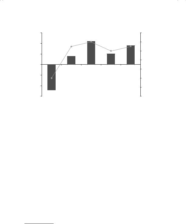
Since many of these studies are at least a decade old, it is worth asking whether the weekday effect persists. Looking at just the daily returns on the S&P 500 from 1981 and 2010 and breaking down the weekday returns by day of the week, we estimated the weekday effect for five-year subperiods in Figure 7.13. Note that to make the comparisons across the periods, we netted out the average daily return over each subperiod from the daily average returns by weekday; thus, the returns on Mondays were, on average, 0.13 percent lower than the average daily returns in the 1981 to 1985 subperiod.
25A. Abraham and D. L. Ikenberry, “The Individual Investor and the Weekend Effect,” Journal of Financial and Quantitative Analysis 29 (1994): 263–277.
236 |
|
|
|
|
|
|
|
|
INVESTMENT PHILOSOPHIES |
|||
0.15% |
|
|
|
|
|
|
|
|
|
|
|
|
|
|
Monday |
|
Tuesday |
|
Wednesday |
|
Thursday |
|
Friday |
|
|
|
|
|
|
|
|
|
|
|||||
|
|
|
|
|
|
|
||||||
|
|
|
|
|
|
|
|
|
|
|
|
|
0.10% |
|
|
|
|
|
|
|
0.05% |
|
|
|
|
|
|
|
0.00% |
|
|
|
|
|
|
|
1981–1985 |
1986–1990 |
1991–1995 |
1996–2000 |
2001–2005 |
2006–2010 |
1981–2010 |
|
–0.05% |
|
|
|
|
|
|
|
–0.10% |
|
|
|
|
|
|
|
–0.15% |
|
|
|
|
|
|
|
F I G U R E 7 . 1 3 |
Returns by Weekday: S&P 500 from 1981 to 2010 |
|
|||||
Source: Standard & Poor’s. |
|
|
|
|
|
||
Interestingly, the weekend effect has been muted for much of the past two decades. In fact, Thursdays and Fridays deliver roughly comparable returns to Mondays over the entire period. One hypothesis that we would offer for the dissipation of the weekday effect is that global listings and virtual trading platforms have allowed trading to become almost round-the-clock. The notion that trading on a stock or an index comes to a complete stop from Friday close to Monday open is almost quaint in today’s marketplace.
V o l u m e P a t t e r n s
Though the random walk hypothesis is silent about the relationship between trading volume and prices, it does assume that all available information is incorporated in the current price. Since trading volume is part of publicly available information, there should therefore be no information value to knowing how many shares were traded yesterday or the day before.
As with prices, there is evidence that trading volume carries information about future stock price changes. Datar, Naik, and Radcliffe show that lowvolume stocks earn higher returns than high-volume stocks, though they
Smoke and Mirrors? Price Patterns, Volume Charts, and Technical Analysis |
237 |
Average Monthly Return in Following 6 Months
1.80%
1.60%
1.40%
1.20%
1.00%
0.80%
0.60%
0.40%
Winners
0.20%
Average
0.00%
Low Volume |
Losers |
Average Volume
High Volume
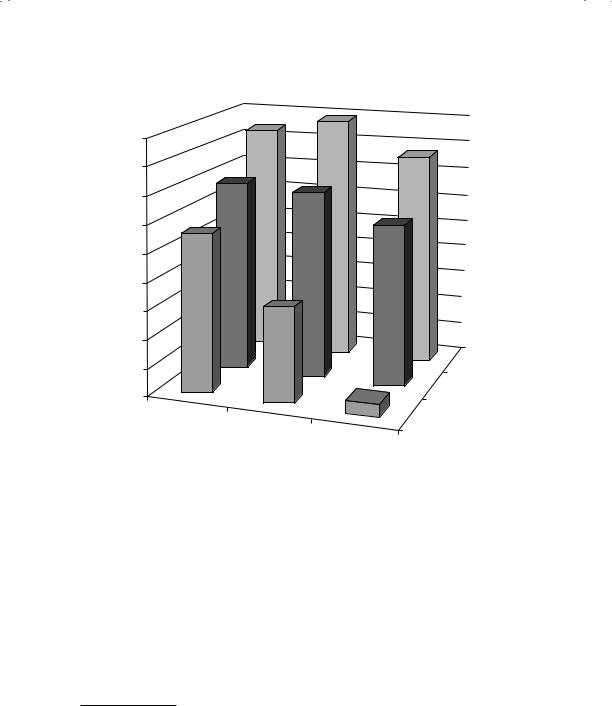
F I G U R E 7 . 1 4 Volume and Price Interaction: NYSE and AMEX Stocks, 1965 to 1995
Source: C. M. C. Lee and B. Swaminathan, “Price Momentum and Trading Volume,” Journal of Finance 5 (2000): 2016–2069.
attribute the differential return to a liquidity premium on the former.26 A more surprising result comes from Lee and Swaminathan, who look at the interrelationship between price and trading volume.27 In particular, they examine the price momentum effect that was documented by Jegadeesh and Titman—that stocks that go up are more likely to keep going up and stocks that go down are more likely to keep dropping in the months after—and show that it is much more pronounced for high-volume stocks. Figure 7.14 classifies stocks based on how well or badly they have done in the past six months (winners, average stocks, and losers) and their trading volume (low,
26V. Datar, N. Naik, and R. Radcliffe, “Liquidity and Asset Returns: An Alternative Test,” Journal of Financial Markets 1 (1998): 205–219.
27C. M. C. Lee and B. Swaminathan, “Price Momentum and Trading Volume,”
Journal of Finance 5 (2000): 2016–2069.

238 |
INVESTMENT PHILOSOPHIES |
average, and high) and looks at returns on these stocks in the following six months.
Note that the price momentum effect is strongest for stocks with high trading volume. In other words, a price increase or decrease that is accompanied by strong volume is more likely to continue into the next period. Stickel and Verecchia confirm this result with shorter-period returns; they conclude that increases in stock prices that are accompanied by high trading volume are more likely to carry over into the next trading day.28
In summary, the level of trading volume in a stock, changes in volume, and volume accompanied by price changes all seem to provide information that investors can use to pick stocks. It is not surprising that trading volume is an integral part of technical analysis.
D A T A M I N I N G O R A N O M A L I E S
When looking at the evidence on seasonal and temporal anomalies in stock price data, we are faced with an interesting dilemma. As stock price data has become both richer (we have gone from annual to intraday data and from just equity markets to bond and derivatives markets) and easier to access and use, it is not surprising that the number of inefficiencies and anomalies discovered has also increased. You could argue that some of these findings can be attributed to the sheer volume of data that is available to us. As hundreds of
researchers pore over this data, using finer and finer microscopes, they will find patterns depending on the portion of the data that they are looking at.
In a spirited defense of efficient markets, Fama presents the argument that almost all of the anomalies and inefficiencies that researchers have detected over the past 40 years can be attributed purely to chance, rather than irrational or inefficient investors. In fact, he makes the interesting point that those researchers who claim to find inefficiencies cannot seem to agree on whether the inefficiencies indicate a market that overreacts or one that underreacts to new information.29
28S. Stickel and R. Verecchia, “Evidence That Trading Volume Sustains Stock Price Changes,” Financial Analysts Journal (November–December 1994): 57–67.
29E. F. Fama, “Market Efficiency, Long-Term Returns, and Behavioral Finance,”
Journal of Financial Economics 49 (September 1998): 283–306.

Smoke and Mirrors? Price Patterns, Volume Charts, and Technical Analysis |
239 |
T H E F O U N D A T I O N S O F T E C H N I C A L A N A L Y S I S
It is best to let technical analysts provide the basis for their approach in their own words. Edwards and Magee, in their classic book on technical analysis, made the following argument:
It is futile to assign an intrinsic value to a stock certificate. One share of U.S. Steel, for example, was worth $261 in the early fall of 1929, but you could buy it for only $22 in June 1932. By March 1937 it was selling for $126 and just one year later for $38. . . . This sort of thing, this wide divergence between presumed value and intrinsic value, is not the exception; it is the rule; it is going on all the time. The fact is that the real value of U.S. Steel is determined at any given time solely, definitely and inexorably by supply and demand, which are accurately reflected in the transactions consummated on the floor of the exchange.30
If we were to summarize the assumptions that underlie technical analysis, we would list the following:
Market value is determined solely by the interaction of supply and demand. We do not think that nonchartists would have any quarrels with this assumption, which describes how prices are set in any market.
Supply and demand are governed by numerous factors, both rational and irrational. The market continually and automatically weighs all these factors. Note that a random walker would have no qualms about this assumption, either, but would point out that any irrational factors are just as likely to be on one side of the market as on the other.
Disregarding minor fluctuations in the market, stock prices tend to move in trends that persist for an appreciable length of time. This is where non-chartists would part ways with chartists. In a rational or even a reasonably sensible market, any trend that can be discerned by investors using charts should provide profit opportunities that when taken advantage of should eliminate the trend.
Changes in trend are caused by shifts in demand and supply. These shifts, no matter why they occur, can be detected sooner or later in the action of the market itself. This is at the core of technical analysis.
30R. Edwards and J. Magee, Technical Analysis of Stock Trends (Boca Raton, FL: St. Lucie Press, 2001).