

aswath_damodaran-investment_philosophies_2012
.pdf120 |
INVESTMENT PHILOSOPHIES |
Net Payoff on
Call Option
If asset value < strike price, you lose what you paid for the call.
Strike Price
Price of Underlying Asset
F I G U R E 4 . 8 Payoff on Call Option
profit. If the value of the asset rises above the exercise price, you will not exercise the right to sell at a lower price. Instead, the option will be allowed to expire without being exercised, resulting in a net loss of the original price paid for the put option. Figure 4.9 summarizes the net payoff on buying a put option.
With both call and put options, the potential for profit to the buyer is significant, but the potential for loss is limited to the price paid for the option.
D e t e r m i n a n t s o f O p t i o n V a l u e
What is it that determines the value of an option? At one level, options have expected cash flows just like all other assets, and that may seem to make them good candidates for discounted cash flow valuation. The two key characteristics of options—that they derive their value from some other
Net Payoff on Put
If asset value > strike price, you lose what you paid for the put.
Strike Price
Price of Underlying Asset
F I G U R E 4 . 9 Payoff on Put Option

Show Me the Money: The Basics of Valuation |
121 |
traded asset, and the fact that their cash flows are contingent on the occurrence of a specific event—do suggest an easier alternative. We can create a portfolio that has the same cash flows as the option being valued, by combining a position in the underlying asset with borrowing or lending. This portfolio is called a replicating portfolio and should cost the same amount as the option. The principle that two assets (the option and the replicating portfolio) with identical cash flows cannot sell at different prices is called the arbitrage principle.
Options are assets that derive value from an underlying asset; increases in the value of the underlying asset will increase the value of the right to buy at a fixed price and reduce the value to sell that asset at a fixed price. Conversely, increasing the strike price will reduce the value of calls and increase the value of puts.
While calls and puts move in opposite directions when stock prices and strike prices are varied, they both increase in value as the life of the option and the variance in the underlying asset’s value increase. This is because the buyers of options have limited losses. Unlike traditional assets that tend to get less valuable as risk is increased, options become more valuable as the underlying asset becomes more volatile. This is so because the added variance cannot worsen the downside risk (you still cannot lose more than what you paid for the option) but increases the potential for higher profits. In addition, a longer option life just allows more time for both call and put options to appreciate in value.
The final two inputs that affect the value of the call and put options are the riskless interest rate and the expected dividends on the underlying asset. Buyers of call and put options usually pay the price of the option up front, and then wait for the expiration day to exercise. There is a present value effect associated with the fact that the promise to buy an asset for $1 million in 10 years is less onerous than paying for it now. Thus, higher interest rates will generally increase the value of call options (by reducing the present value of the price on exercise) and decrease the value of put options (by decreasing the present value of the price received on exercise). The expected dividends paid by assets make them less valuable; thus, the call option on a stock that does not pay a dividend should be worth more than a call option on a stock that does pay a dividend. The reverse should be true for put options.
C O N C L U S I O N
In this chapter, we laid the foundations for the models that we will be using to value both assets and firms in the coming chapters. There are three classes

122 |
INVESTMENT PHILOSOPHIES |
of valuation models. The most general of these models, discounted cash flow valuation, can be used to value any asset with expected cash flows over its life. The value is the present value of the expected cash flows at a discount rate that reflects the riskiness of the cash flows, and this principle applies whether one is looking at a zero coupon government bond or equity in highrisk firms. Relative valuation models are a second set of models, where we value assets based on how similar assets are priced by the market. Third, there are some assets that generate cash flows only in the event of a specified contingency, and these assets will not be valued accurately using discounted cash flow models. Instead, they should be viewed as options and valued using option pricing models.
E X E R C I S E S
Pick a company that you are familiar with, in terms of its business and history. Try the following:
1.Do an intrinsic valuation of a company. You can build your own spreadsheet or use one of mine (check under spreadsheets on my website). Here are some of your choices:
a.A simple dividend discount model (for valuing financial service companies).
b.A simple FCFE model (for valuing companies, using cash flows to equity).
c.A simple FCFF model (for valuing companies, using cash flows to the firm).
2.Pick a multiple (P/E, price to book, value/EBITDA) and compare how your company is priced relative to the sector and to other companies within the sector. If your company trades at a much higher or lower multiple than other companies, can you think of reasons why it should?
3.Assuming that you have done both intrinsic and relative valuation, are the values similar? If not, how would you explain the difference?
Lessons for Investors
All assets that generate or are expected to generate cash flows can be valued by discounting the expected cash flows back at a rate that reflects the riskiness of the cash flows—more risky cash flows should be discounted at higher rates.

Show Me the Money: The Basics of Valuation |
123 |
The value of an ongoing business is a function of four variables—how much the business generates in cash flows from existing investments, how long these cash flows can be expected to grow at a rate higher than the growth rate of the economy (high-growth period), the level of the growth rate during this period, and the riskiness of the cash flows. Companies with higher cash flows, higher growth rates, longer high-growth periods, and lower risk will have higher values.
Alternatively, assets can be valued by looking at how similar assets are priced in the market. This approach is called relative valuation and is built on the presumption that the market is correct, on average.
Assets whose cash flows are contingent on the occurrence of specific events are called options and can be valued using option pricing models.


CHAPTER 5
Many a Slip: Trading,
Execution, and Taxes
A s investors consider different investment strategies, they have to take into account two important factors that can determine whether these strategies pay off—trading costs and taxes. It costs to trade, and some strategies create larger trading costs than others. The costs of trading clearly impose a drag on the performance of all active investors and can turn otherwise winning portfolios into losing portfolios. As we debate the extent of these costs, we need to get a measure of what the costs are, how they vary across investment strategies, and how investors can minimize these costs. In this chapter, we take an expansive view of trading costs and argue that the brokerage cost is only one and often the smallest component of trading costs. We also look at the trading costs associated with holding real assets (such as real estate) and nontraded investments (like equity in a private business). In addition, we discuss the trade-off between trading costs and
trading speed.
There is a second equally important element in investment success. Investors get to take home after-tax returns and not before-tax returns. Thus, strategies that perform well before taxes may be money losers after taxes. Taxes are particularly difficult to deal with, partly because they can vary across investors and across investments for the same investor, and partly because the tax code itself changes over time, often in unpredictable ways. We will consider the evidence that many mutual funds do their investors a disservice by not considering taxes and that after-tax returns lag pretax returns considerably at these funds. We will also look at ways in which we can adjust our investment strategies to keep tax liabilities low.
T H E T R A D I N G C O S T D R A G
While we debate what constitutes trading costs and how to measure them, there is a fairly simple way in which we can estimate, at the minimum,
125

126 |
INVESTMENT PHILOSOPHIES |
how much trading costs affect the returns of the average portfolio manager. Active money managers trade because they believe that there is profit in trading, and the return to any active money manager has three ingredients to it:
Return on active money manager
= Expected returnRisk + Return from active trading − Trading costs
Looking across all active money managers, we can reasonably assume that the average expected return across all of them has to be equal to the return on the market index, at least in a market like the United States, where institutional investors hold 60 percent or more of all shares outstanding. Thus, subtracting the the return on the index from the average return made by active money managers should give us a measure of the payoff to active money management:
Average returnActive Money Managers − Return on index = Returns from active trading − Trading costs
Here the evidence becomes quite depressing. The average active money manager has underperformed the index in the past decade by about 1 percent. If we take the view that active trading adds no excess return on average, the trading costs, at the minimum, should be 1 percent of the portfolio on an annual basis. If we take the view that active trading does add to the returns, the trading costs will be greater than 1 percent of the portfolio on an annual basis.
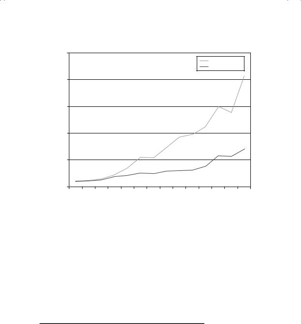
There are also fairly specific examples of real portfolios that have been constructed to replicate hypothetical portfolios, where the magnitude of the trading costs is illustrated starkly. For decades, Value Line has offered advice to individual investors on what stocks to buy and which ones to avoid, and has ranked stocks from 1 to 5 based on their desirability as investments. Studies by academics and practitioners found that Value Line rankings seemed to correlate with actual returns. In 1979, Value Line decided to create a mutual fund that would invest in the stocks that it was recommending to its readers. In Figure 5.1, we consider the difference in returns in the 1979 to 1991 time period between the fund that Value Line ran and the paper portfolio that Value Line has used to compute the returns that its stock picks would have had.
The paper portfolio had an annual return of 26.2 percent, whereas the Value Line fund had a return of 16.1 percent. While part of the difference can be attributed to Value Line waiting until its subscribers had a chance to
Many a Slip: Trading, Execution, and Taxes |
127 |
|
$2,500 |
|
Paper Portfolio |
|
Real Fund |
|
$2,000 |
in 1978 |
|
$100 Invested |
$1,500 |
$1,000 |
|
Value of |
$500 |
|
|
|
$0 |
|
1978 1979 1980 1981 1982 1983 1984 1985 1986 1987 1988 1989 1990 1991 |
Year
F I G U R E 5 . 1 Value Line—Paper Portfolio versus Real Fund
trade, a significant portion of the difference can be explained by the costs of trading.
Looking at the evidence, there are a couple of conclusions that we would draw. The first is that money managers collectively either underestimate trading costs or overestimate the returns to active trading, or both. The second is that trading costs are a critical ingredient to any investment strategy, and can make the difference between a successful strategy and an unsuccessful one.
T H E C O M P O N E N T S O F T R A D I N G C O S T S : T R A D E D
F I N A N C I A L A S S E T S
There are some investors who undoubtedly operate under the misconception that the only cost of trading stocks is the brokerage commission that they pay when they buy or sell assets. While this might be the only cost that they pay explicitly, there are other costs that they incur in the course of trading that generally dwarf the commission cost. When trading any asset, they are three other ingredients that go into the trading costs. The first is the spread

128 |
INVESTMENT PHILOSOPHIES |
between the price at which you can buy an asset (the ask price) and the price at which you can sell the same asset at the same point in time (the bid price). The second is the price impact that an investor can create by trading on an asset, pushing the price up when buying the asset and pushing it down while selling. The third cost, which was first proposed by Jack Treynor in an article on transaction costs, is the opportunity cost associated with waiting to trade.1 Although being a patient trader may reduce the first two components of trading cost, the waiting can cost profits both on trades that are made and in terms of trades that would have been profitable if made instantaneously but become unprofitable as a result of the waiting. It is the sum of these costs that makes up the total trading cost on an investment strategy.
T h e B i d - A s k S p r e a d
There is a difference between what a buyer will pay and the seller will receive, at the same point in time for the same asset, in almost every traded asset market. The bid-ask spread refers to this difference. In the section that follows, we examine why this difference exists, how large it is as a cost, the determinants of its magnitude, and its effects on returns in different investment strategies.
W h y I s T h e r e a B i d - A s k S p r e a d ? In most markets, there is a dealer or market maker who sets the bid-ask spread, and there are three types of costs that the dealer faces that the spread is designed to cover. The first is the risk and the cost of holding inventory, the second is the cost of processing orders, and the final cost is the cost of trading with more informed investors. The spread has to be large enough to cover these costs and yield a reasonable profit to the market maker on his or her investment in the profession.
The Inventory Rationale Consider market makers or specialists on the floor of the exchange who have to quote bid prices and ask prices at which they are obligated to execute buy and sell orders from investors.2 These investors, themselves, could be trading because of information they have received (informed traders), for liquidity (liquidity traders), or based on their belief that an asset is undervalued or overvalued (value traders). In
1J. Treynor, “What Does It Take to Win the Trading Game?” Financial Analysts Journal (January–February 1981).
2Y. Amihud and H. Mendelson, “Asset Pricing and the Bid-Ask Spread,” Journal of Financial Economics 17 (1986): 223–249.

Many a Slip: Trading, Execution, and Taxes |
129 |
such a market, if the market makers set the bid price too high, they will accumulate an inventory of the stock. If market makers set the ask price too low, they will find themselves with a large short position in the stock. In either case, there is a cost to the market makers that they will attempt to recover by increasing the spread between the bid and ask prices.
Market makers also operate with inventory constraints, some of which are externally imposed (by the exchanges or regulatory agencies) and some of which are internally imposed (due to capital limitations and risk). As the market makers’ inventory positions deviate from their optimal positions, they bear a cost and will try to adjust the bid and ask prices to get back to their preferred positions.
The Processing Cost Argument Since market makers incur a processing cost when executing orders, the bid-ask spread has to cover, at the minimum, these costs. While these costs are likely to be very small for large orders of stocks traded on the exchanges, they become larger for small orders of stocks that might be traded only through a dealership market. Furthermore, since a large proportion of this cost is fixed, these costs as a percentage of the price will generally be higher for low-priced stocks than for high-priced stocks.
Technology clearly has reduced the processing cost associated with trades as computerized systems take over from traditional record keepers. These cost reductions should be greatest for stocks where the bulk of the trades are small trades—small stocks held by individual rather than institutional investors.
The Adverse Selection Problem The adverse selection problem arises from the different motives investors have for trading on an asset—liquidity, information, and views on valuation. Since investors do not announce their reasons for trading at the time of the trade, the market maker always runs the risk of trading against more informed investors. Since market makers can expect to lose on such trades, they have to charge an average spread that is large enough to compensate for such losses. This theory would suggest that spreads will be a function of three factors:
1.The proportion of informed traders in an asset market. As the proportion of informed traders in a market increases, the probability that the market maker will trade with an informed investor on the next trade also increases, pushing the bid-ask spread up.
2.The differential information possessed, on average, by these traders. The greater the differences in information possessed by different investors, the more the market maker has to worry about the magnitude of the impact.